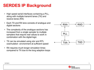
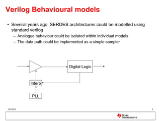
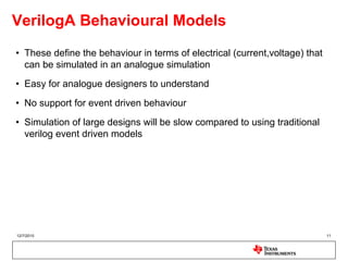
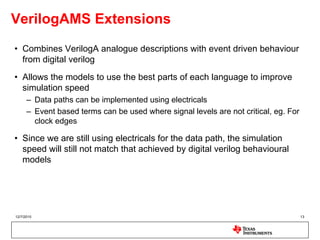
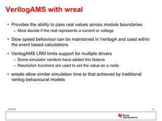
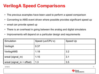
Analogue Behavioural Modelling:
An Inconvenient Truth
Dave Wiltshire, Texas Instruments


12/7/2010                           1
Introduction
• SERDES IP Background
• Verilog behavioural modelling
• VerilogA behavioural modelling
• Behavioural model validation


12/7/2010                          2
SERDES IP Background
• High speed serial interfaces containing a PLL,
  along with multiple transmit lanes (TX) and
  receive lanes (RX)
• Each TX and RX lane consists of analogue and
  digital sections                                 RXA   RXD

• The complexity of the analogue sections has
  increased from a single sampler to multiple
  samplers that require real values to work in     PLL
  combination with the digital logic
• TX can be simulated using xtor and RTL
                                                   TXA   TXD
  cosimulation environment at sufficient speed
• RX requires much longer simulation times
  compared to TX due to the long adaption loops


12/7/2010                                                      3
SERDES RX Architecture


12/7/2010                4
Verilog Behavioural models
• Several years ago, SERDES architectures could be modelled using
  standard verilog
      – Analogue behaviour could be isolated within individual models
      – The data path could be implemented as a simple sampler


                                    Digital Logic


               Interp


                PLL


12/7/2010                                                               5
Verilog Behavioural models
• Complexity of SERDES architectures is increasing
      – Digitally controlled analogue circuits are now required
            • Now require adaptive equalisation and level control
      – This drives the need to pass analogue signals around the design
      – Verilog historically has not supported using real values for ports


                    EQ                                     Digital Logic


                                   Interp


                                    PLL

12/7/2010                                                                    6
Hierarchical Connections
• Use upwards name references to identify a real value in another
  module
• Standard verilog code that does not require any special capabilities
• Can be difficult to maintain when the design changes


12/7/2010                                                                7
Hierarchical Connection Example
module test;

fred ifred   (.fred_input (fred_input),
              .fred_output (fred_output));
jimmy ijimmy (.jimmy_input (fred_output),
              .jimmy_output (jimmy_output));
                                               module jimmy (jimmy_input,jimmy_output);
endmodule
                                               input    jimmy_input;
module fred (fred_input,fred_output);          output   jimmy_output;

input fred_input;                              real     jimmy_real_input;
output fred_output;                            real     jimmy_real_internal;

real        fred_real_output;                  assign   jimmy_output = jimmy_input;

assign fred_output = fred_input;               always
                                                 begin
always @(fred_output)                            jimmy_real_input    = fred.fred_real_output;
  begin                                          jimmy_real_internal = 0.5*jimmy_real_input;
  fred_real_output = 1.0*fred_output;            @(fred.fred_real_output);
  end                                            end

endmodule                                      endmodule


12/7/2010                                                                                 8
Connection using Verilog PLI
• PLI can be used to trace a normal signal back to it’s source driver
• A local real variable is used to pass the required data between the two
  end points


                    fred_output                     jimmy_input


 fred_output_real                                          jimmy_input_real


12/7/2010                                                                     9
PLI Connection Example
module test;

fred ifred   (.fred_input (fred_input),
              .fred_output (fred_output));     module jimmy (jimmy_input,jimmy_output);
jimmy ijimmy (.jimmy_input (fred_output),
              .jimmy_output (jimmy_output));   input    jimmy_input;
                                               output   jimmy_output;
endmodule
                                               real     jimmy_input_real;
module fred (fred_input,fred_output);          real     jimmy_real_internal;

input fred_input;                              assign      jimmy_output = jimmy_input;
output fred_output;
                                               initial
real        fred_output_real;                    begin
                                                 $connect_real(jimmy_input);
buf (fred_output,fred_input);                    end

always @(fred_output)                          always @(jimmy_input_real)
  begin                                          begin
  fred_output_real = 1.0*fred_output;            jimmy_real_internal = 0.5*jimmy_input_real;
  end                                            end

endmodule                                      endmodule


12/7/2010                                                                                 10
VerilogA Behavioural Models
• These define the behaviour in terms of electrical (current,voltage) that
  can be simulated in an analogue simulation
• Easy for analogue designers to understand
• No support for event driven behaviour
• Simulation of large designs will be slow compared to using traditional
  verilog event driven models


12/7/2010                                                                    11
VerilogA example
module example (clk, signal_in, offset, q, vdd, vss);
input clk;
input signal_in;
input offset;
input vdd,vss;
output q;

electrical clk, signal_in, offset, vdd, vss, q;

real vth, state;

analog
  begin
  vth = 0.5 * V(vdd,vss);
  @(cross(V(clk)-vth,+1))
    begin
    if (V(signal_in,vss) > V(offset,vss)) state = V(vdd,vss);
    else                                  state = V(vss);
    end
  V(q,vss) <+ transition(state,30p,10p);
  end

endmodule


12/7/2010                                                       12
VerilogAMS Extensions
• Combines VerilogA analogue descriptions with event driven behaviour
  from digital verilog
• Allows the models to use the best parts of each language to improve
  simulation speed
      – Data paths can be implemented using electricals
      – Event based terms can be used where signal levels are not critical, eg. For
        clock edges

• Since we are still using electricals for the data path, the simulation
  speed will still not match that achieved by digital verilog behavioural
  models


12/7/2010                                                                             13
VerilogAMS Example
module example (clk, signal_in, offset, q, vdd, vss);
input clk;
input signal_in;
input offset;
input vdd,vss;
output q;

electrical signal_in, offset, vdd, vss;

reg state;

always @(posedge clk)
  begin
  if (V(signal_in,vss) > V(offset,vss)) state = 1’b1;
  else                                  state = 1’b0;
  end

assign q = state;

endmodule


12/7/2010                                               14
VerilogAMS with wreal
• Provides the ability to pass real values across module boundaries
      – Must decide if the real represents a current or voltage

• Slow speed behaviour can be maintained in VerilogA and used within
  the event based calculations
• VerilogAMS LRM limits support for multiple drivers
      – Some simulator vendors have added this feature
      – Resolution functions are used to set the value on a node

• wreals allow similar simulation time to that achieved by traditional
  verilog behavioural models


12/7/2010                                                                15
VerilogAMS with wreal Example
module example (clk, signal_in, offset, q, vdd, vss);
input clk;
input signal_in;
input offset;
input vdd,vss;
output q;

wreal      signal_in;
electrical offset, vdd, vss;

reg state;

always @(posedge clk)
  begin
  if (signal_in > V(offset,vss))   state = 1’b1;
  else                             state = 1’b0;
  end

assign q = state;

endmodule


12/7/2010                                               16
VerilogA Speed Comparisons
• The previous examples have been used to perform a speed comparison
• Converting to AMS event driven where possible provides significant speed up
• wreal can provide speed up
• There is an overhead in going between the analog and digital simulators
• Improvements will depend on a particular design and requirements

Simulation                   Speed (us/CPU s)         Speed Up

VerilogA                     0.37

VerilogAMS                   1.18                     3.2

wreal (signal_in)            1.15                     3.1

wreal (signal_in + offset)   1.3                      3.5
12/7/2010                                                                       17
Behavioural Model Validation
• Behavioural models need to be checked against their transistor
  implementations
• A testplan should be generated to document and track required tests
      – Target correct functionality for the behavioural models against the

• The tests identified in the testplan should be run on a regular basis to
  identify any divergence between the model and the implementation


12/7/2010                                                                     18
Summary
• VerilogA provides a very good behavioural modelling environment for
  mixed signal designs
• Modelling requirements should be considered early in the design cycle
      – Help to drive the architecture to one that makes modelling easier
      – Consider how individual signals will be modelled for best performance
            • Use event based constructs wherever possible
      – Solutions will be dependant on the specific design requirements
            • Simulation speed can go down as well as up!

• Testplans and model verification environments should be implemented
  and maintained to ensure the models match the design


12/7/2010                                                                       19

Analogue Behavioral Modelling: An Inconvenient Truth

  • 1.
    Analogue Behavioural Modelling: AnInconvenient Truth Dave Wiltshire, Texas Instruments 12/7/2010 1
  • 2.
    Introduction • SERDES IPBackground • Verilog behavioural modelling • VerilogA behavioural modelling • Behavioural model validation 12/7/2010 2
  • 3.
    SERDES IP Background •High speed serial interfaces containing a PLL, along with multiple transmit lanes (TX) and receive lanes (RX) • Each TX and RX lane consists of analogue and digital sections RXA RXD • The complexity of the analogue sections has increased from a single sampler to multiple samplers that require real values to work in PLL combination with the digital logic • TX can be simulated using xtor and RTL TXA TXD cosimulation environment at sufficient speed • RX requires much longer simulation times compared to TX due to the long adaption loops 12/7/2010 3
  • 4.
  • 5.
    Verilog Behavioural models •Several years ago, SERDES architectures could be modelled using standard verilog – Analogue behaviour could be isolated within individual models – The data path could be implemented as a simple sampler Digital Logic Interp PLL 12/7/2010 5
  • 6.
    Verilog Behavioural models •Complexity of SERDES architectures is increasing – Digitally controlled analogue circuits are now required • Now require adaptive equalisation and level control – This drives the need to pass analogue signals around the design – Verilog historically has not supported using real values for ports EQ Digital Logic Interp PLL 12/7/2010 6
  • 7.
    Hierarchical Connections • Useupwards name references to identify a real value in another module • Standard verilog code that does not require any special capabilities • Can be difficult to maintain when the design changes 12/7/2010 7
  • 8.
    Hierarchical Connection Example moduletest; fred ifred (.fred_input (fred_input), .fred_output (fred_output)); jimmy ijimmy (.jimmy_input (fred_output), .jimmy_output (jimmy_output)); module jimmy (jimmy_input,jimmy_output); endmodule input jimmy_input; module fred (fred_input,fred_output); output jimmy_output; input fred_input; real jimmy_real_input; output fred_output; real jimmy_real_internal; real fred_real_output; assign jimmy_output = jimmy_input; assign fred_output = fred_input; always begin always @(fred_output) jimmy_real_input = fred.fred_real_output; begin jimmy_real_internal = 0.5*jimmy_real_input; fred_real_output = 1.0*fred_output; @(fred.fred_real_output); end end endmodule endmodule 12/7/2010 8
  • 9.
    Connection using VerilogPLI • PLI can be used to trace a normal signal back to it’s source driver • A local real variable is used to pass the required data between the two end points fred_output jimmy_input fred_output_real jimmy_input_real 12/7/2010 9
  • 10.
    PLI Connection Example moduletest; fred ifred (.fred_input (fred_input), .fred_output (fred_output)); module jimmy (jimmy_input,jimmy_output); jimmy ijimmy (.jimmy_input (fred_output), .jimmy_output (jimmy_output)); input jimmy_input; output jimmy_output; endmodule real jimmy_input_real; module fred (fred_input,fred_output); real jimmy_real_internal; input fred_input; assign jimmy_output = jimmy_input; output fred_output; initial real fred_output_real; begin $connect_real(jimmy_input); buf (fred_output,fred_input); end always @(fred_output) always @(jimmy_input_real) begin begin fred_output_real = 1.0*fred_output; jimmy_real_internal = 0.5*jimmy_input_real; end end endmodule endmodule 12/7/2010 10
  • 11.
    VerilogA Behavioural Models •These define the behaviour in terms of electrical (current,voltage) that can be simulated in an analogue simulation • Easy for analogue designers to understand • No support for event driven behaviour • Simulation of large designs will be slow compared to using traditional verilog event driven models 12/7/2010 11
  • 12.
    VerilogA example module example(clk, signal_in, offset, q, vdd, vss); input clk; input signal_in; input offset; input vdd,vss; output q; electrical clk, signal_in, offset, vdd, vss, q; real vth, state; analog begin vth = 0.5 * V(vdd,vss); @(cross(V(clk)-vth,+1)) begin if (V(signal_in,vss) > V(offset,vss)) state = V(vdd,vss); else state = V(vss); end V(q,vss) <+ transition(state,30p,10p); end endmodule 12/7/2010 12
  • 13.
    VerilogAMS Extensions • CombinesVerilogA analogue descriptions with event driven behaviour from digital verilog • Allows the models to use the best parts of each language to improve simulation speed – Data paths can be implemented using electricals – Event based terms can be used where signal levels are not critical, eg. For clock edges • Since we are still using electricals for the data path, the simulation speed will still not match that achieved by digital verilog behavioural models 12/7/2010 13
  • 14.
    VerilogAMS Example module example(clk, signal_in, offset, q, vdd, vss); input clk; input signal_in; input offset; input vdd,vss; output q; electrical signal_in, offset, vdd, vss; reg state; always @(posedge clk) begin if (V(signal_in,vss) > V(offset,vss)) state = 1’b1; else state = 1’b0; end assign q = state; endmodule 12/7/2010 14
  • 15.
    VerilogAMS with wreal •Provides the ability to pass real values across module boundaries – Must decide if the real represents a current or voltage • Slow speed behaviour can be maintained in VerilogA and used within the event based calculations • VerilogAMS LRM limits support for multiple drivers – Some simulator vendors have added this feature – Resolution functions are used to set the value on a node • wreals allow similar simulation time to that achieved by traditional verilog behavioural models 12/7/2010 15
  • 16.
    VerilogAMS with wrealExample module example (clk, signal_in, offset, q, vdd, vss); input clk; input signal_in; input offset; input vdd,vss; output q; wreal signal_in; electrical offset, vdd, vss; reg state; always @(posedge clk) begin if (signal_in > V(offset,vss)) state = 1’b1; else state = 1’b0; end assign q = state; endmodule 12/7/2010 16
  • 17.
    VerilogA Speed Comparisons •The previous examples have been used to perform a speed comparison • Converting to AMS event driven where possible provides significant speed up • wreal can provide speed up • There is an overhead in going between the analog and digital simulators • Improvements will depend on a particular design and requirements Simulation Speed (us/CPU s) Speed Up VerilogA 0.37 VerilogAMS 1.18 3.2 wreal (signal_in) 1.15 3.1 wreal (signal_in + offset) 1.3 3.5 12/7/2010 17
  • 18.
    Behavioural Model Validation •Behavioural models need to be checked against their transistor implementations • A testplan should be generated to document and track required tests – Target correct functionality for the behavioural models against the • The tests identified in the testplan should be run on a regular basis to identify any divergence between the model and the implementation 12/7/2010 18
  • 19.
    Summary • VerilogA providesa very good behavioural modelling environment for mixed signal designs • Modelling requirements should be considered early in the design cycle – Help to drive the architecture to one that makes modelling easier – Consider how individual signals will be modelled for best performance • Use event based constructs wherever possible – Solutions will be dependant on the specific design requirements • Simulation speed can go down as well as up! • Testplans and model verification environments should be implemented and maintained to ensure the models match the design 12/7/2010 19