Download as PDF, PPTX

![Linear Regression Continued
1 In Equation 1, β0, β1 are two unknown constants, also known as
parameters.
2 Our objective is to use training data and estimate the values of ˆβ0, ˆβ1
3 So far we have discussed the case of simple linear regression. In case
of multiple linear regression, our linear regression model takes the
form
y = β0 + β1x1 + β2x2 + . . . + βpxp + (2)
4 A commonly used technique to find the estimates of the
co-efficients(parameters) is least square method [1].
Ananda Swarup Das A Note on Ridge Regression October 16, 2016 3 / 16](https://image.slidesharecdn.com/ridgeregression-161016121454/85/Ridge-regression-3-320.jpg)
![The Bias-Variance Trade Off
As stated in [1], the expected value of the residual error (yi − ˆf (xi )) is
given by
E(yi − ˆf (xi ))2
= Var(ˆf (xi )) + [Bias(ˆf (xi ))]2
+ Var( ) (4)
1 In the above equation, the first term on the right hand side denotes
the variance of the model that is the amount by which ˆf would
change if the parameters β1, . . . , βp are estimated using different
training data.
2 The second term denotes the error introduced by approximating a
may-be complicated real-life model with a simpler model.
Ananda Swarup Das A Note on Ridge Regression October 16, 2016 5 / 16](https://image.slidesharecdn.com/ridgeregression-161016121454/85/Ridge-regression-5-320.jpg)
![The Bias-Variance Trade Off Continued
Also shown in [1], the expected value of residual error (yi − ˆf (xi )) can also
be expressed as
E(yi − ˆf (xi ))2
= E(f (xi ) + − ˆf (xi ))2
= [f (xi ) − ˆf (xi )]2
+ Var( ) (5)
Notice that we have replace yi = f (xi ) + . The first part [f (xi ) − ˆf (xi )]2
is reducible and we want our estimation of parameters be such that ˆf (xi )
is as close as possible to f (xi ). However, the Var( ) is irreducible.
Ananda Swarup Das A Note on Ridge Regression October 16, 2016 6 / 16](https://image.slidesharecdn.com/ridgeregression-161016121454/85/Ridge-regression-6-320.jpg)
![What do we reduce
1 Reconsider the Equation 4,
E(yi − ˆf (xi ))2 = Var(ˆf (xi )) + [Bias(ˆf (xi ))]2 + Var( ), the expected
value of MSE cannot be less than Var( ).
2 Thus, we have to try to reduce the variance and the bias for the
model ˆf .
Ananda Swarup Das A Note on Ridge Regression October 16, 2016 7 / 16](https://image.slidesharecdn.com/ridgeregression-161016121454/85/Ridge-regression-7-320.jpg)
![The Significance of the choice of λ
1 Stated in [1], for every value of λ there exists a constant s such that
the problem of ridge regression coefficient estimation boils down to
minimize
n
i=1
(yi − β0 −
p
j=1
βj xi,j )2
(6)
s.t p
j=1 β2
j ≤ s
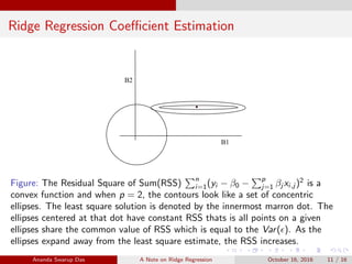
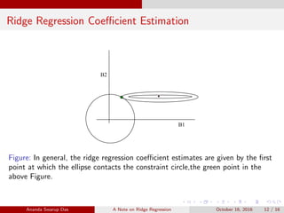
2 Notice that if p = 2, under the constaint p
j=1 β2
j ≤ s, ridge
regression coefficient estimation is equivalent to finding the
coefficients lying within a circle (in general a sphere) centered at the
origin and is of radius
√
s, such that the Equation 6 is minimized.
Ananda Swarup Das A Note on Ridge Regression October 16, 2016 10 / 16](https://image.slidesharecdn.com/ridgeregression-161016121454/85/Ridge-regression-10-320.jpg)
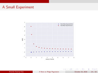

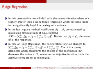
Ridge regression is a technique used for linear regression when the number of predictor variables is greater than the number of observations. It addresses the problem of overfitting by adding a regularization term to the loss function that shrinks large coefficients. This regularization term penalizes coefficients with large magnitudes, improving the model's generalization. Ridge regression finds a balance between minimizing training error and minimizing the size of coefficients by introducing a tuning parameter lambda. The document includes an experiment demonstrating how different lambda values affect the variance and mean squared error of the ridge regression model.


![[Deck] What's New in Spark-Iceberg Integration via DSV2.pptx](https://cdn.slidesharecdn.com/ss_thumbnails/deckwhatsnewinspark-icebergintegrationviadsv2-260210005337-25955b12-thumbnail.jpg?width=640&height=640&fit=bounds)


