Download as PDF, PPTX

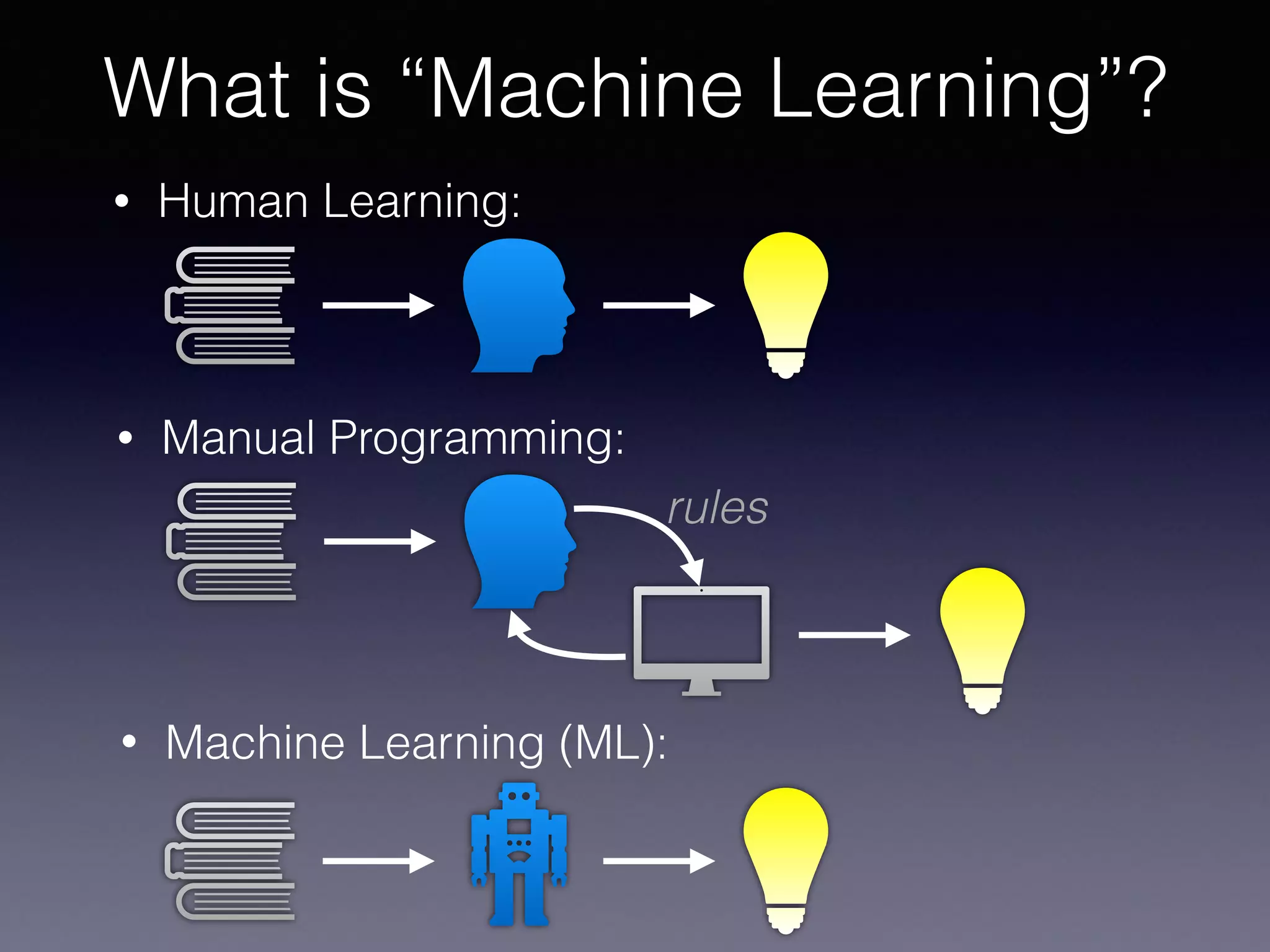
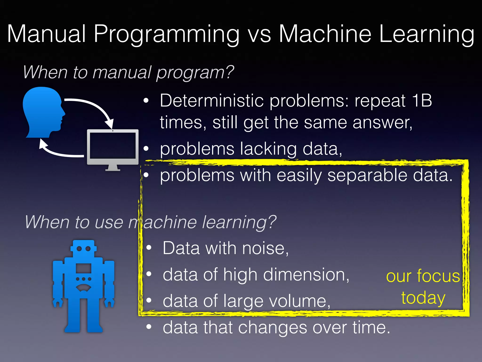
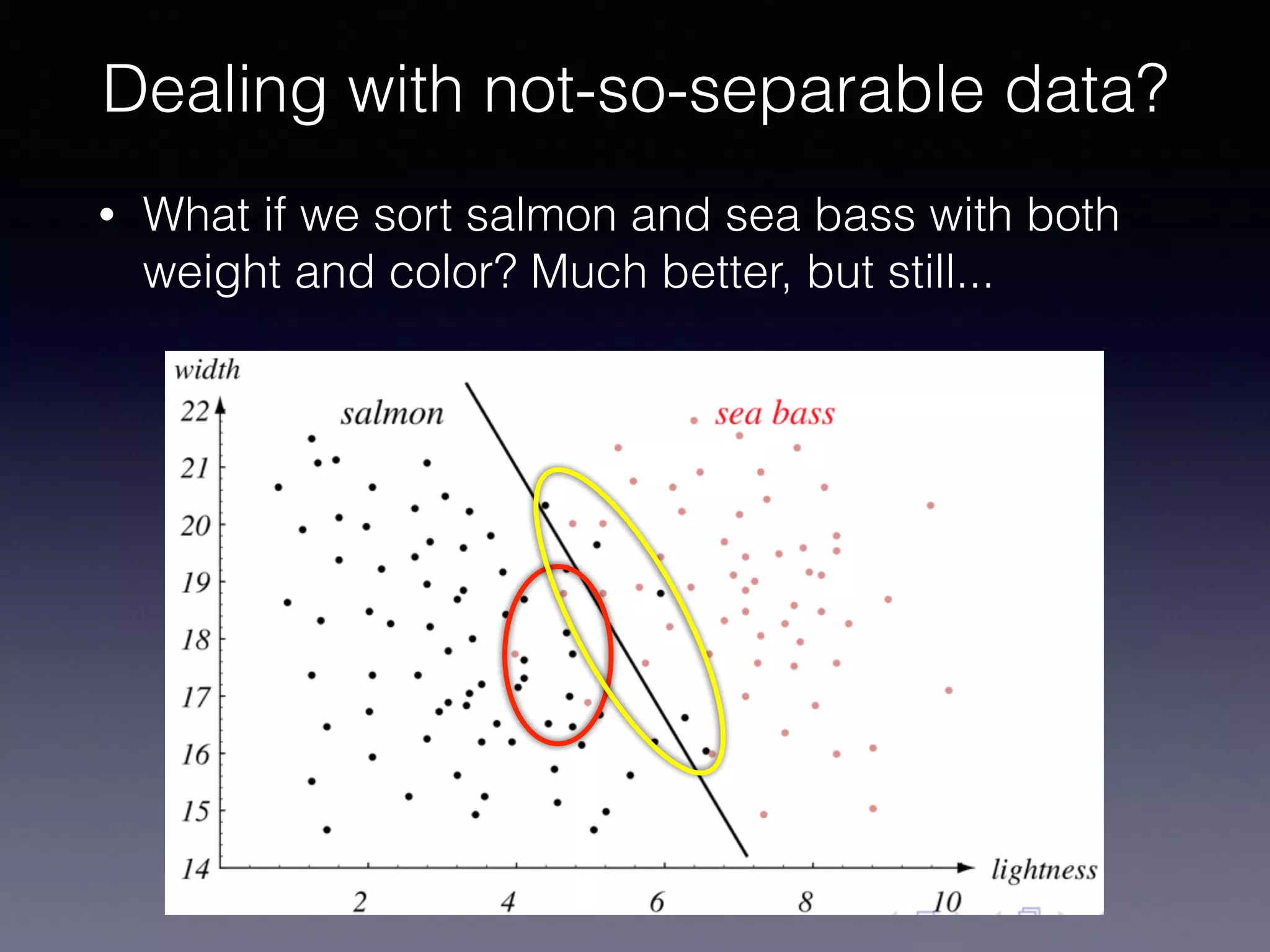
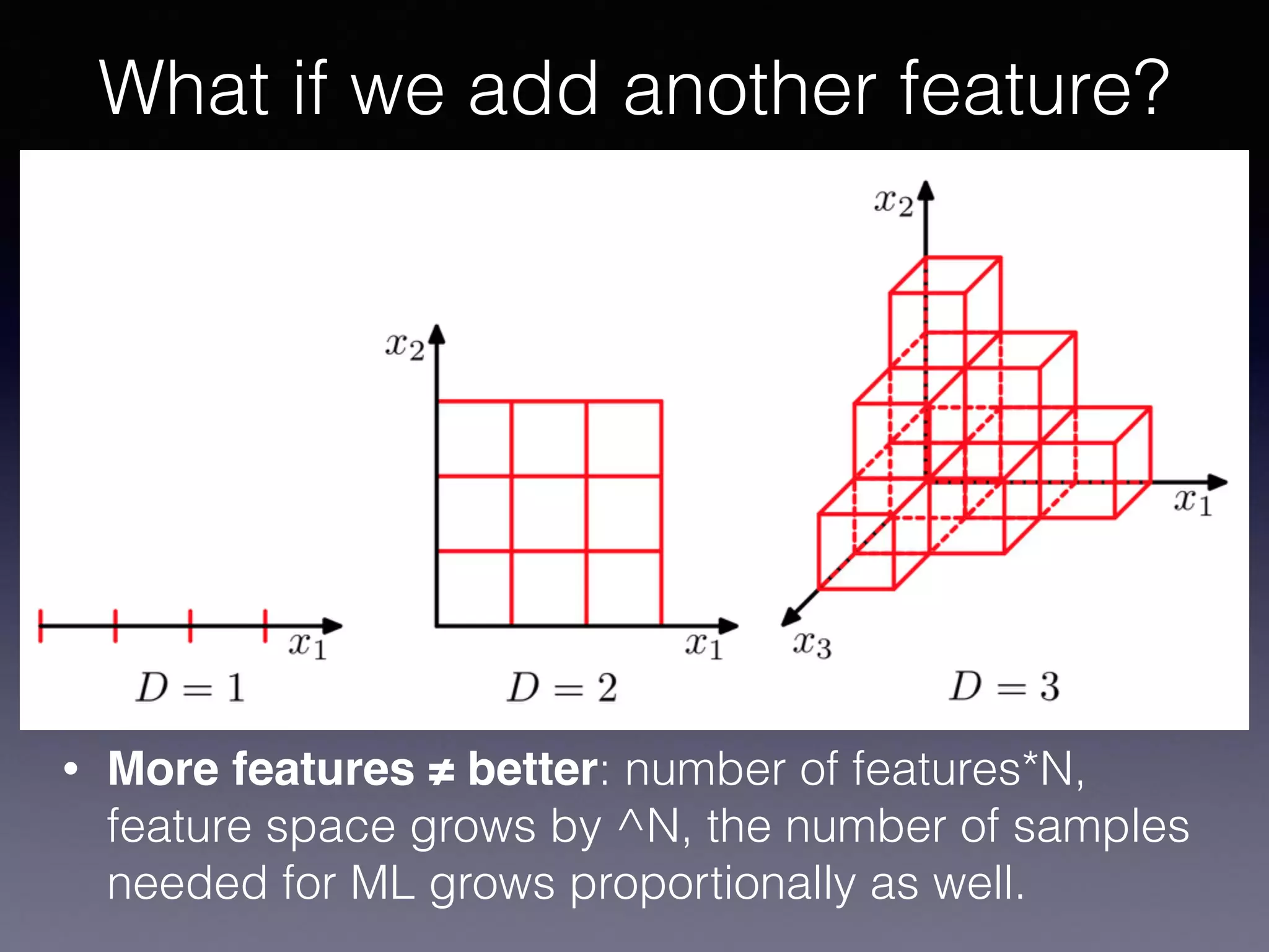
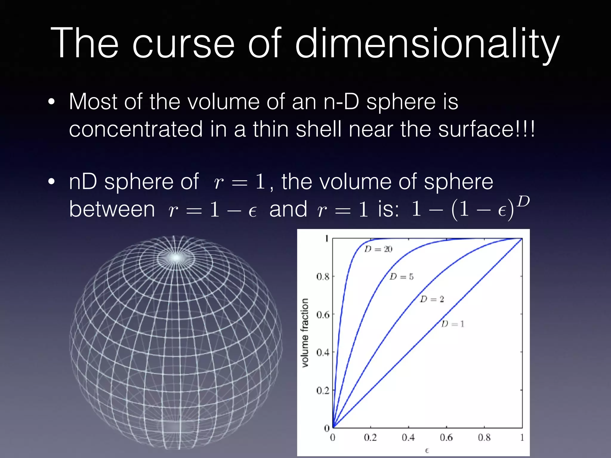
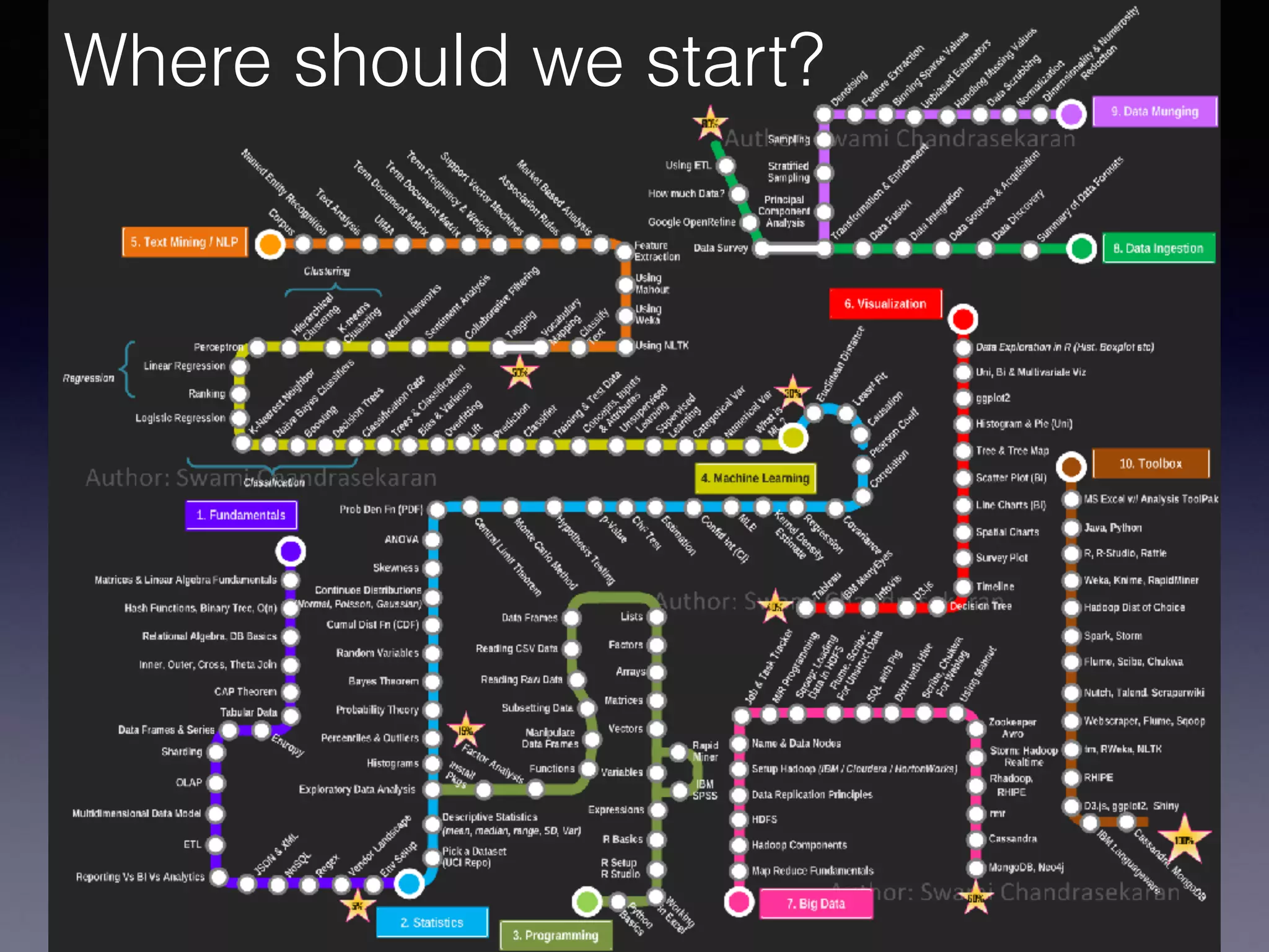
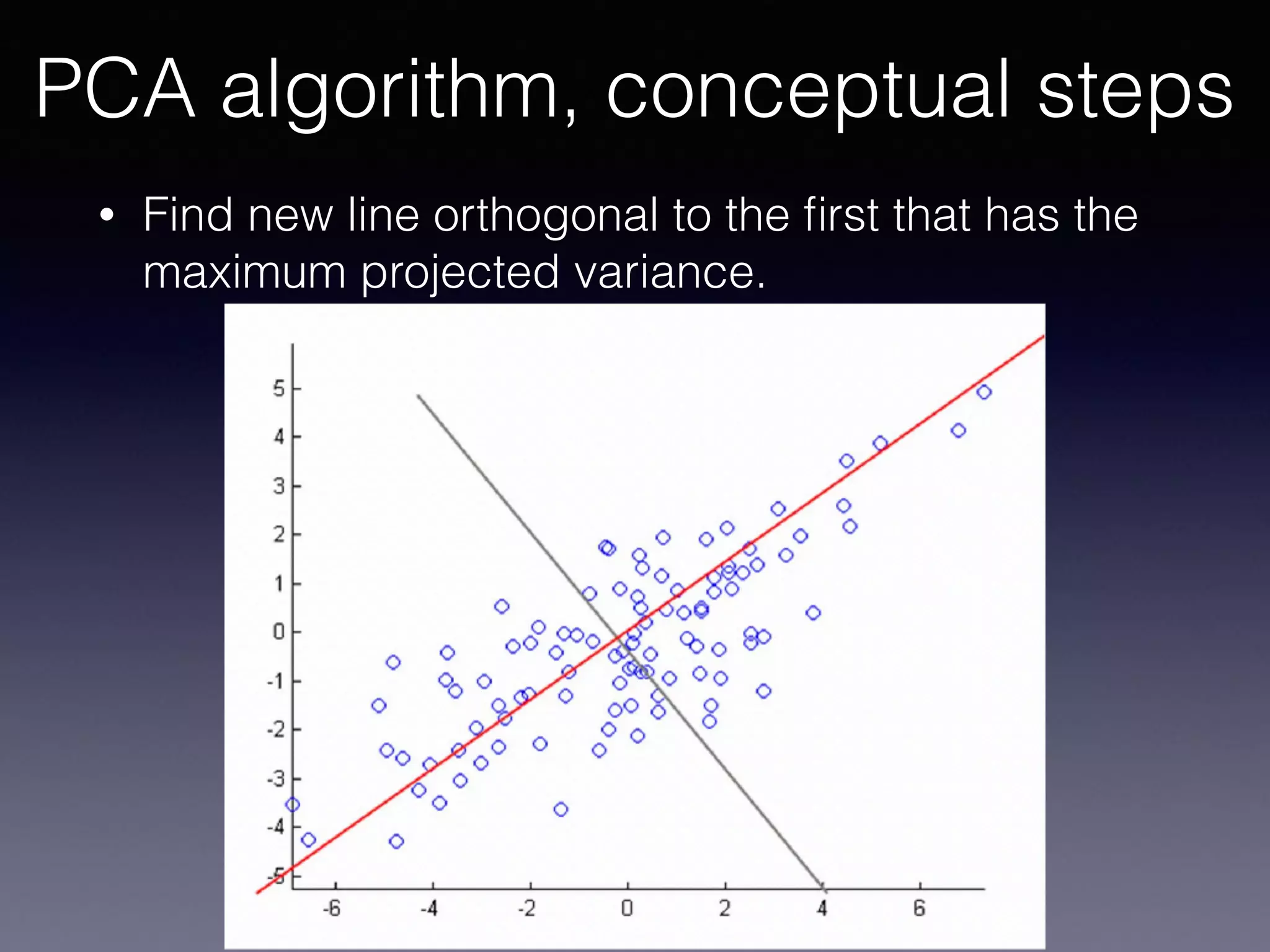
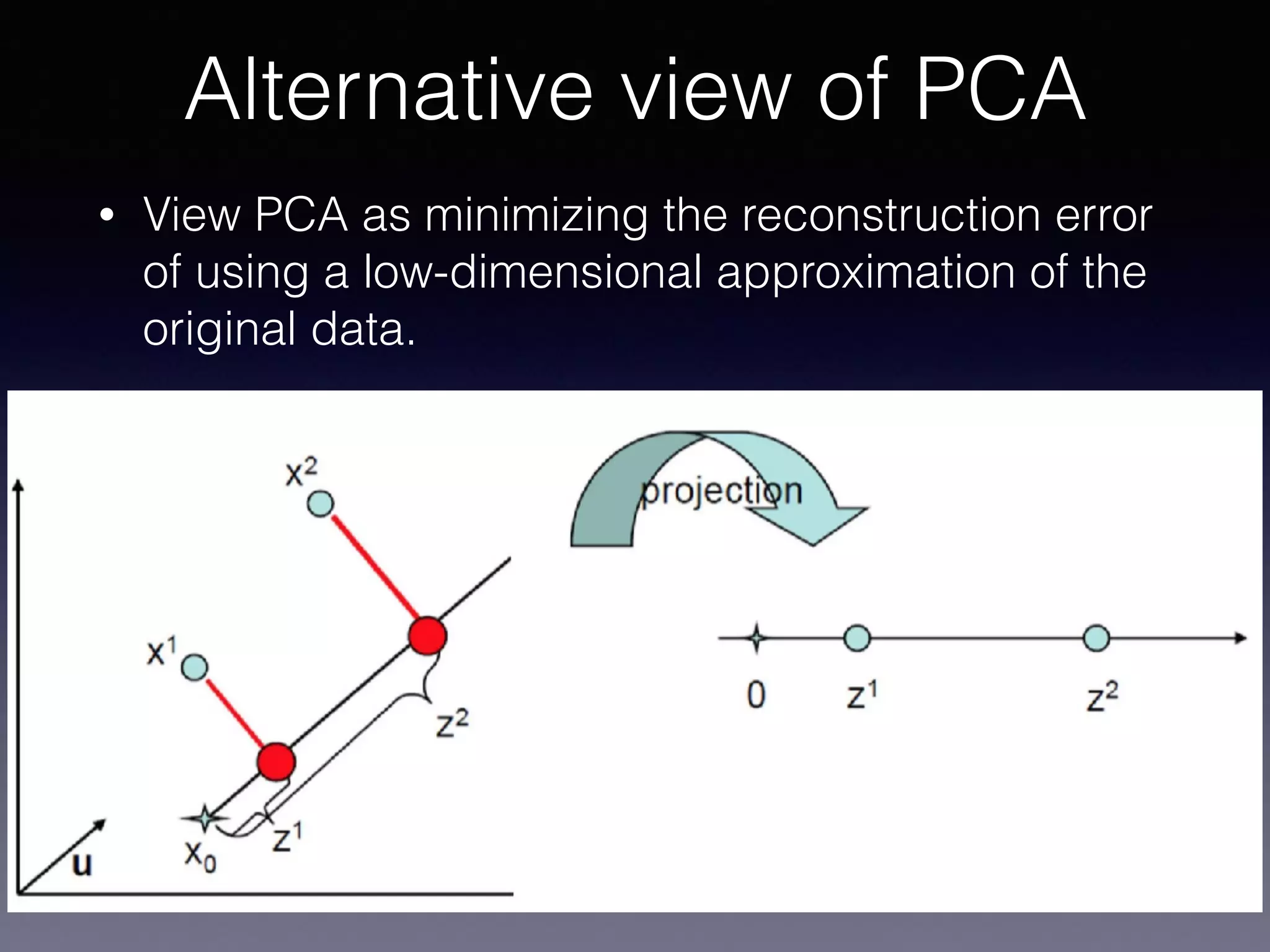
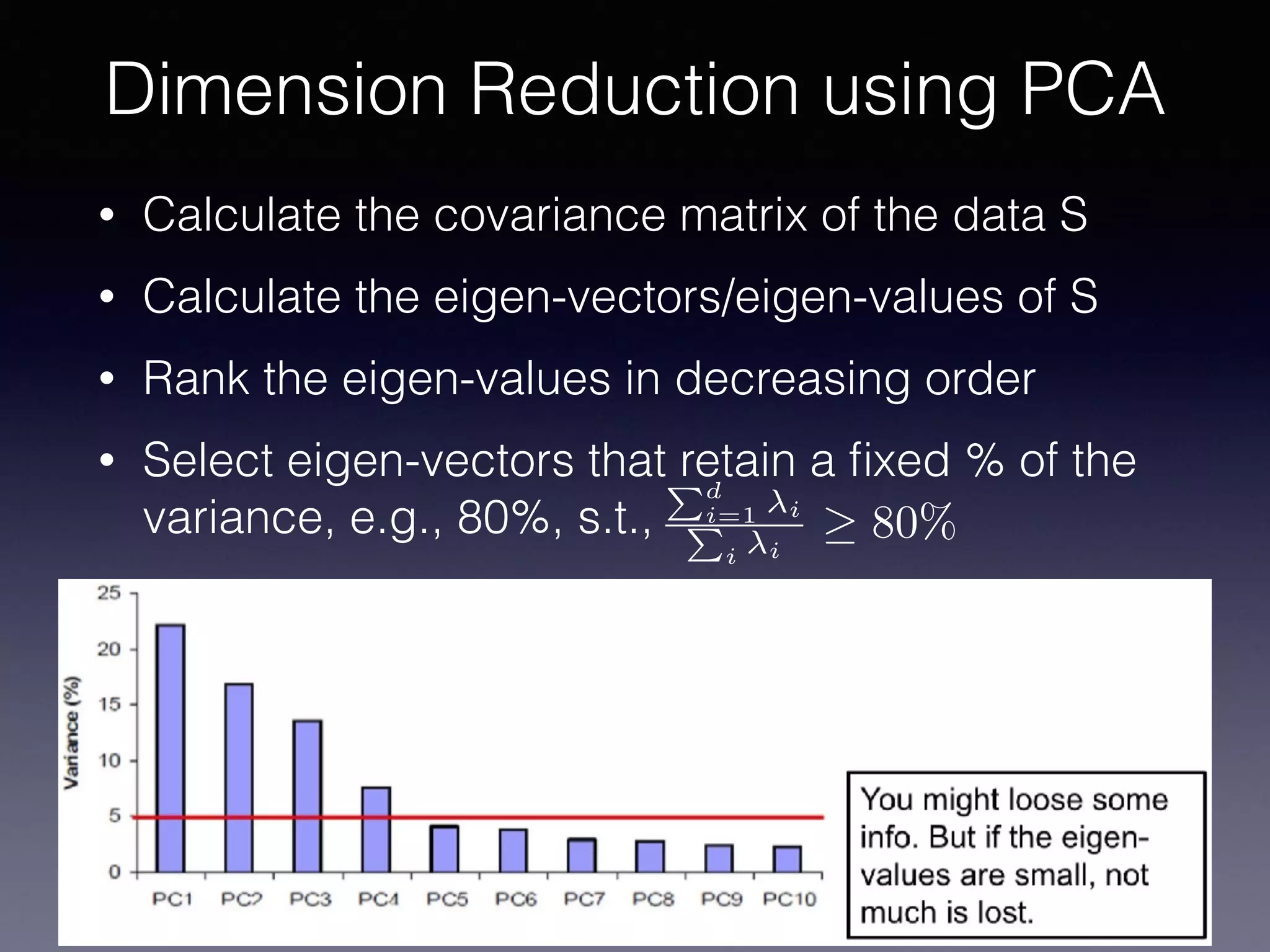
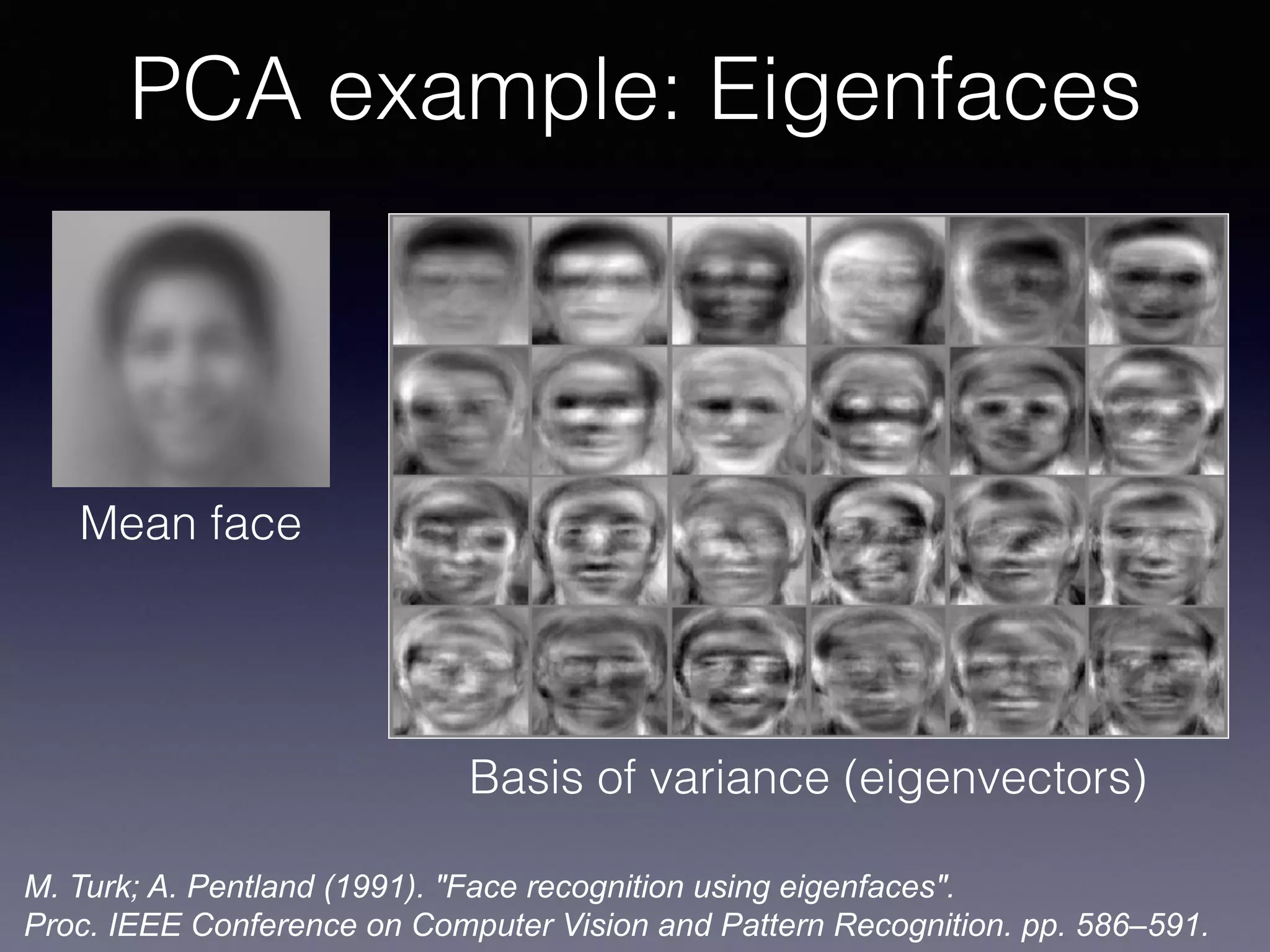
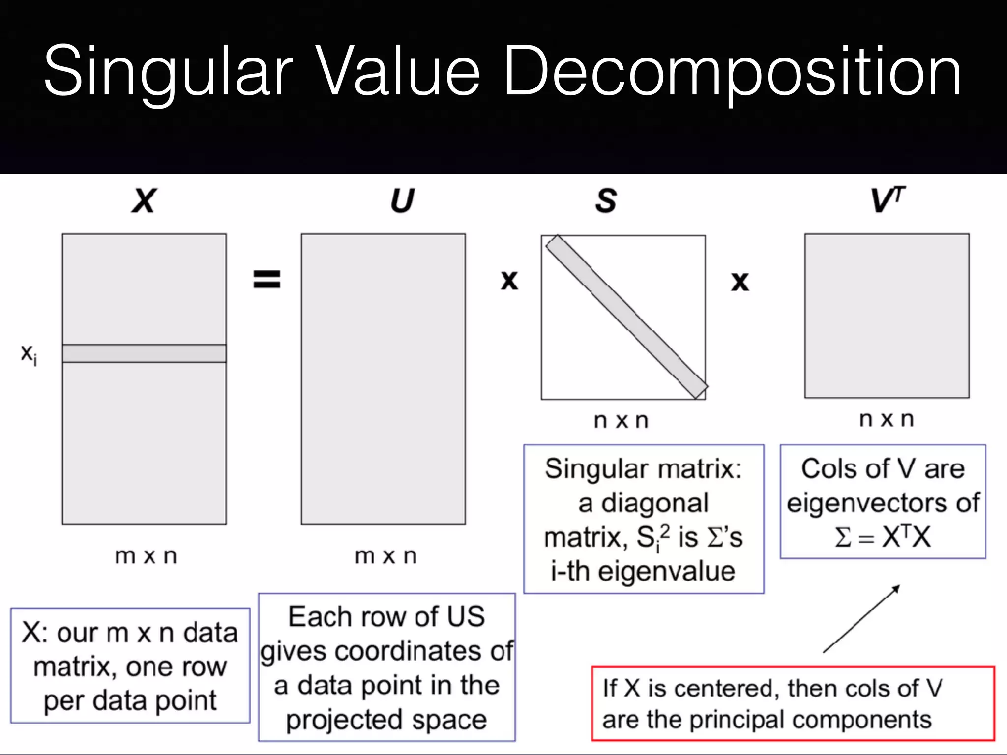
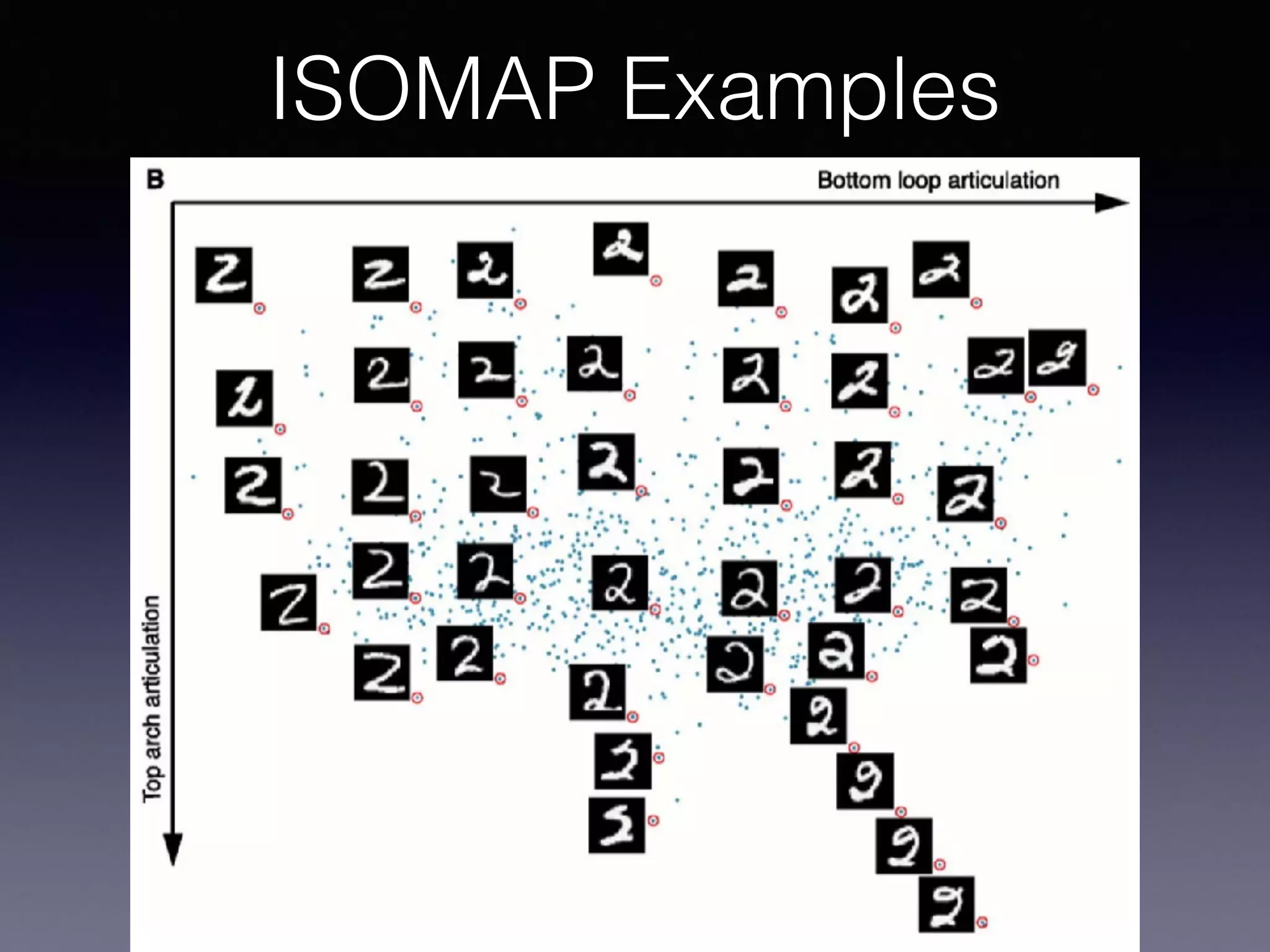
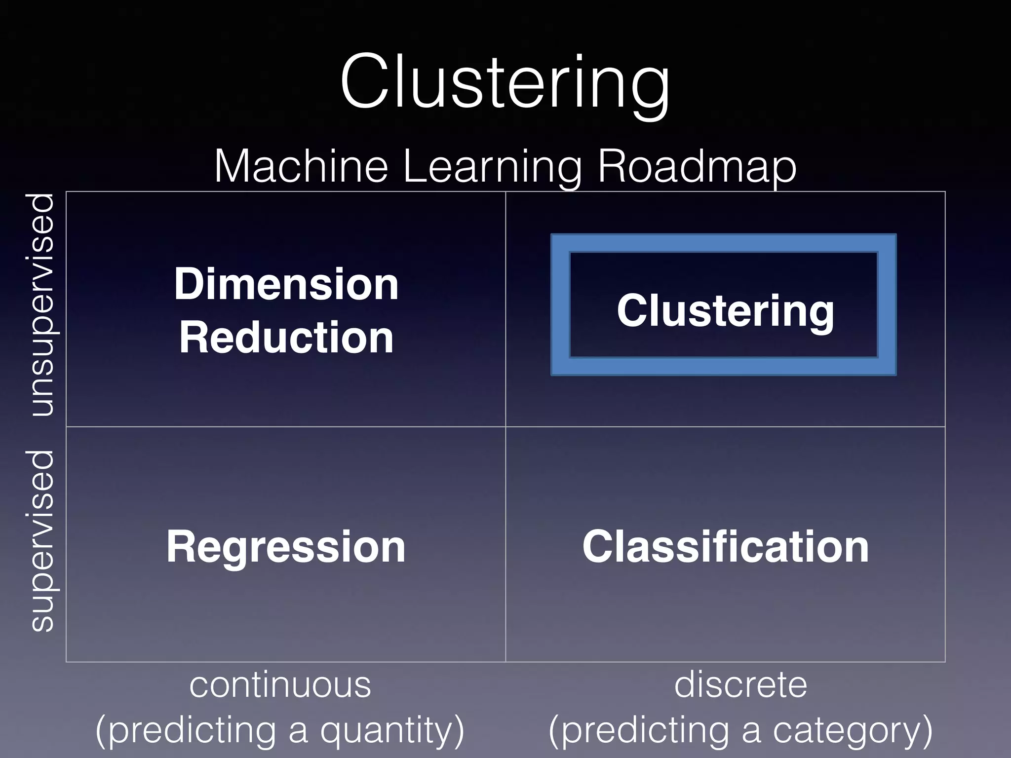
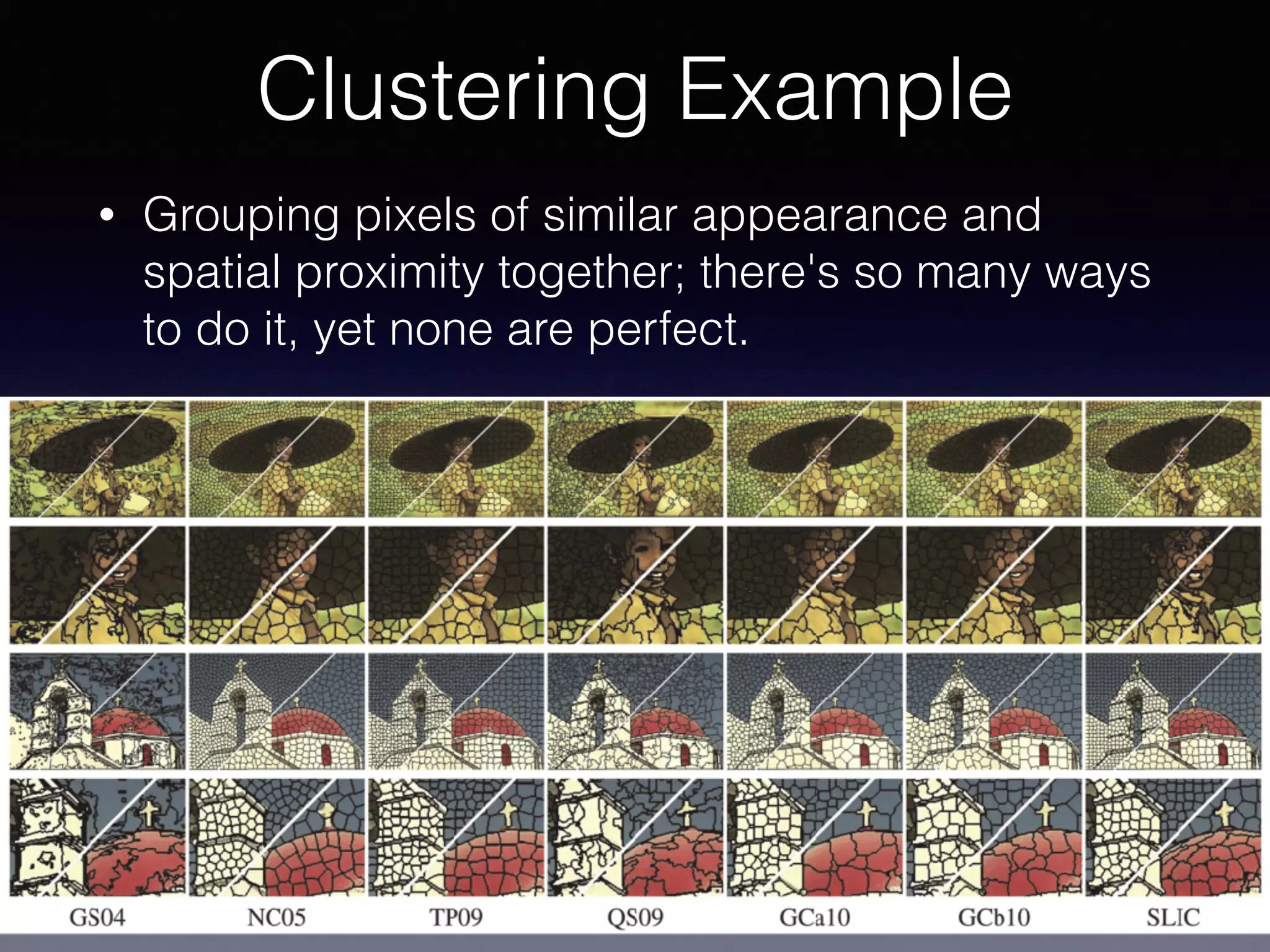
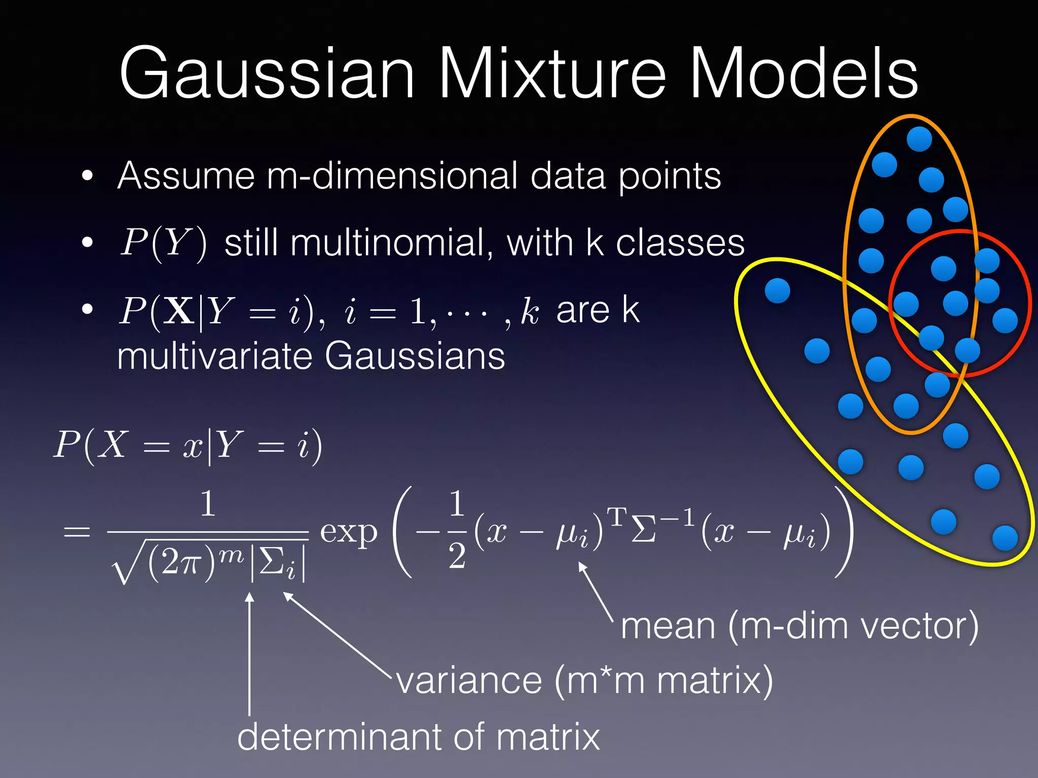
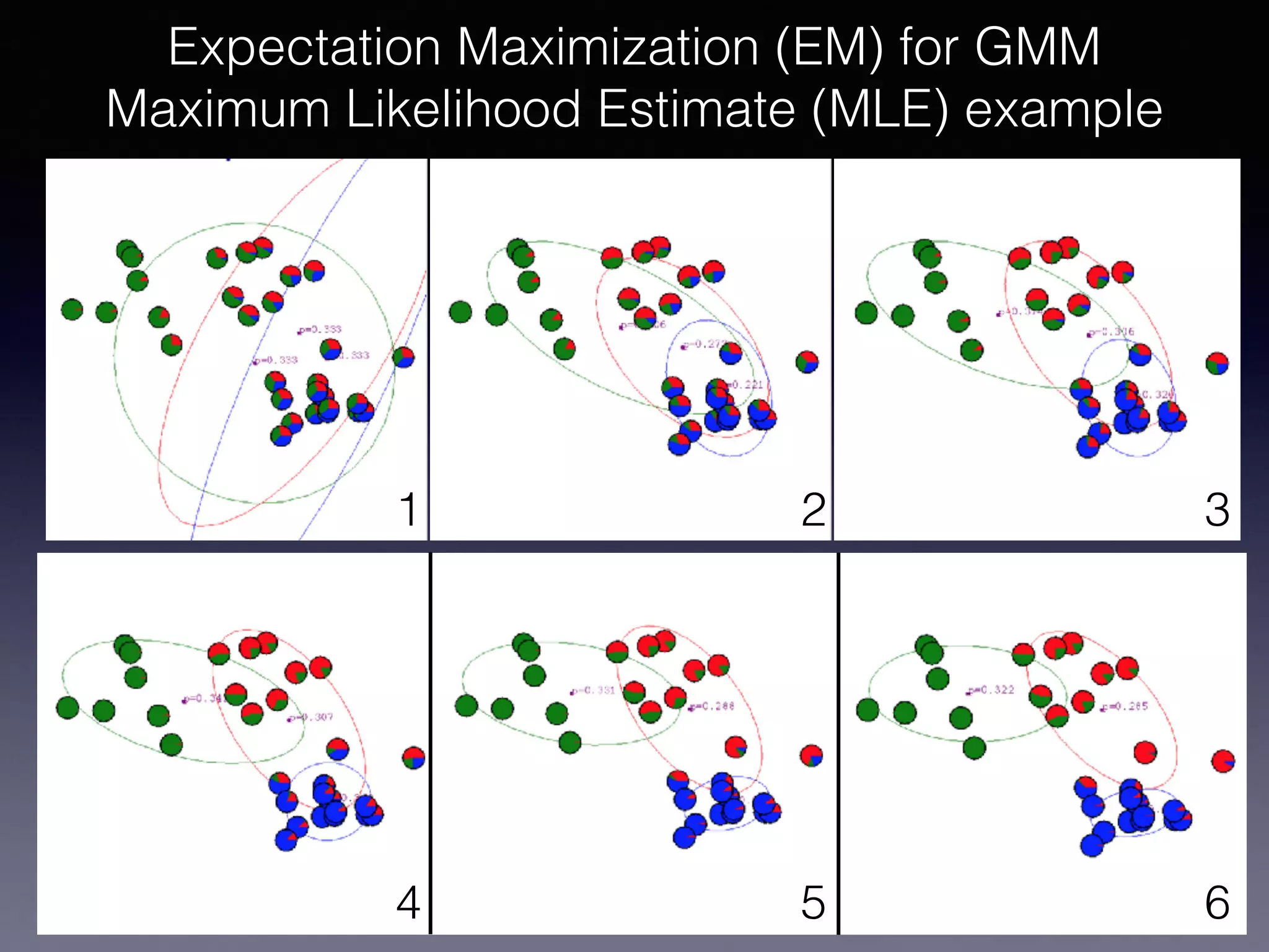
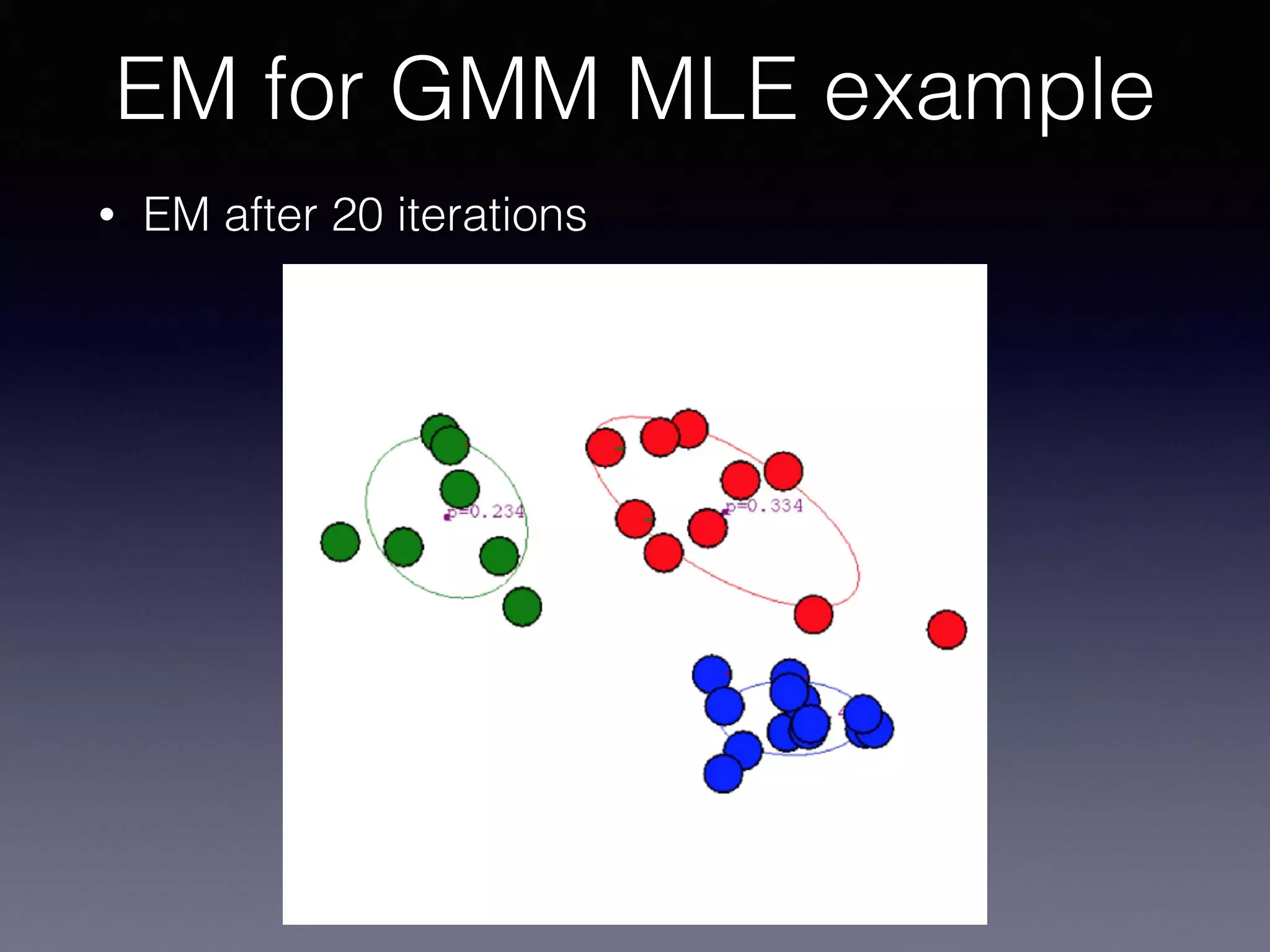
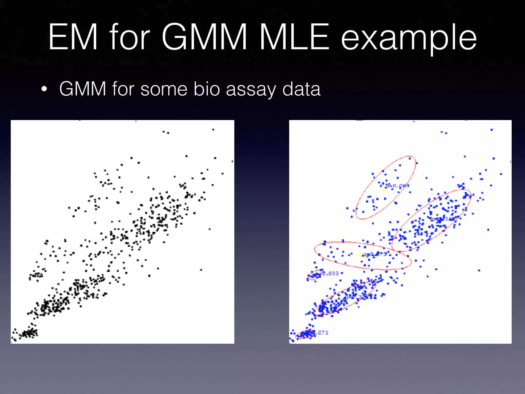
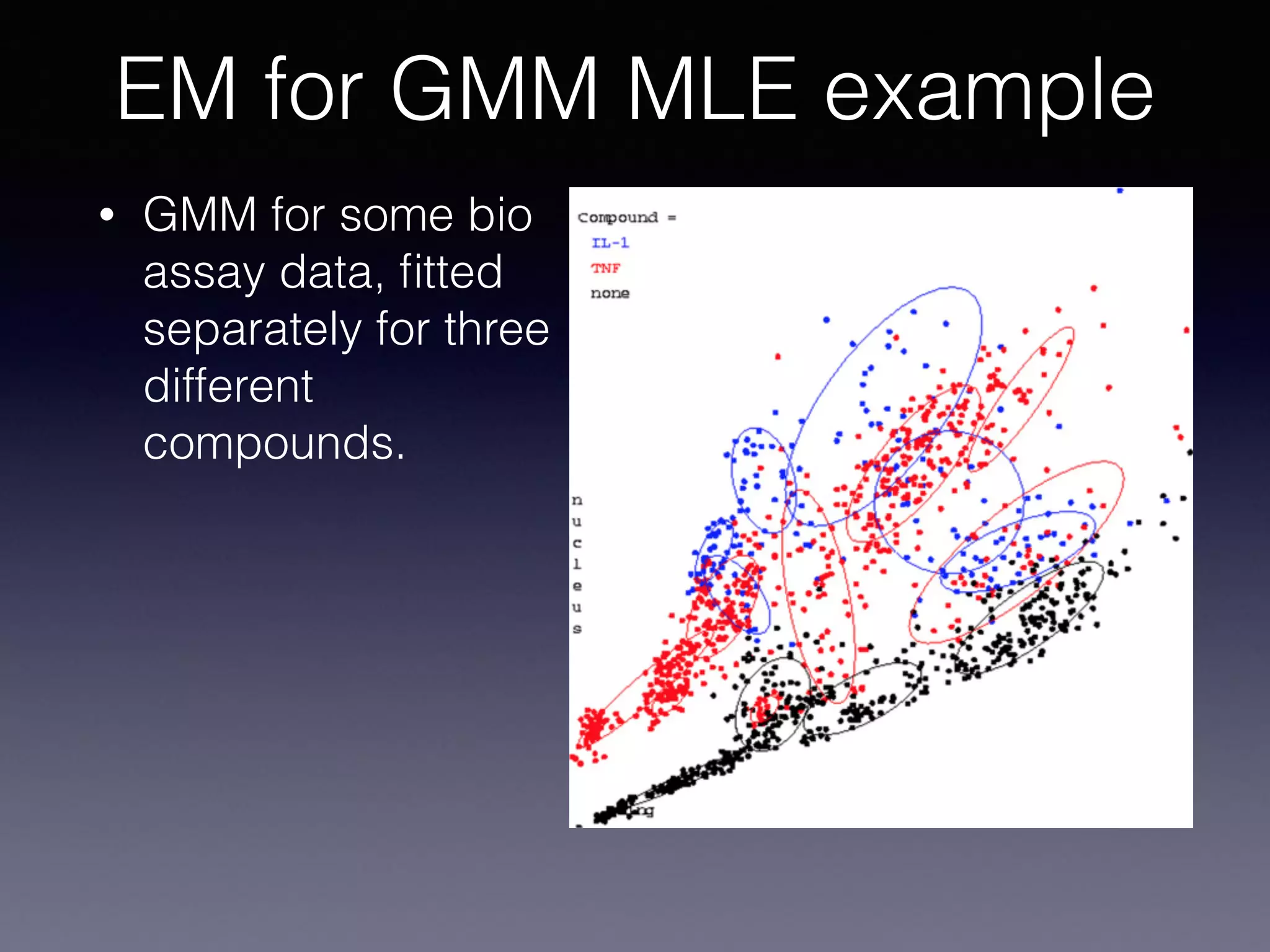
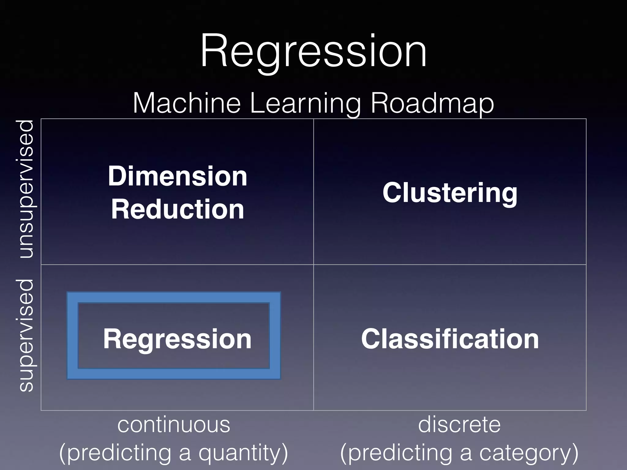
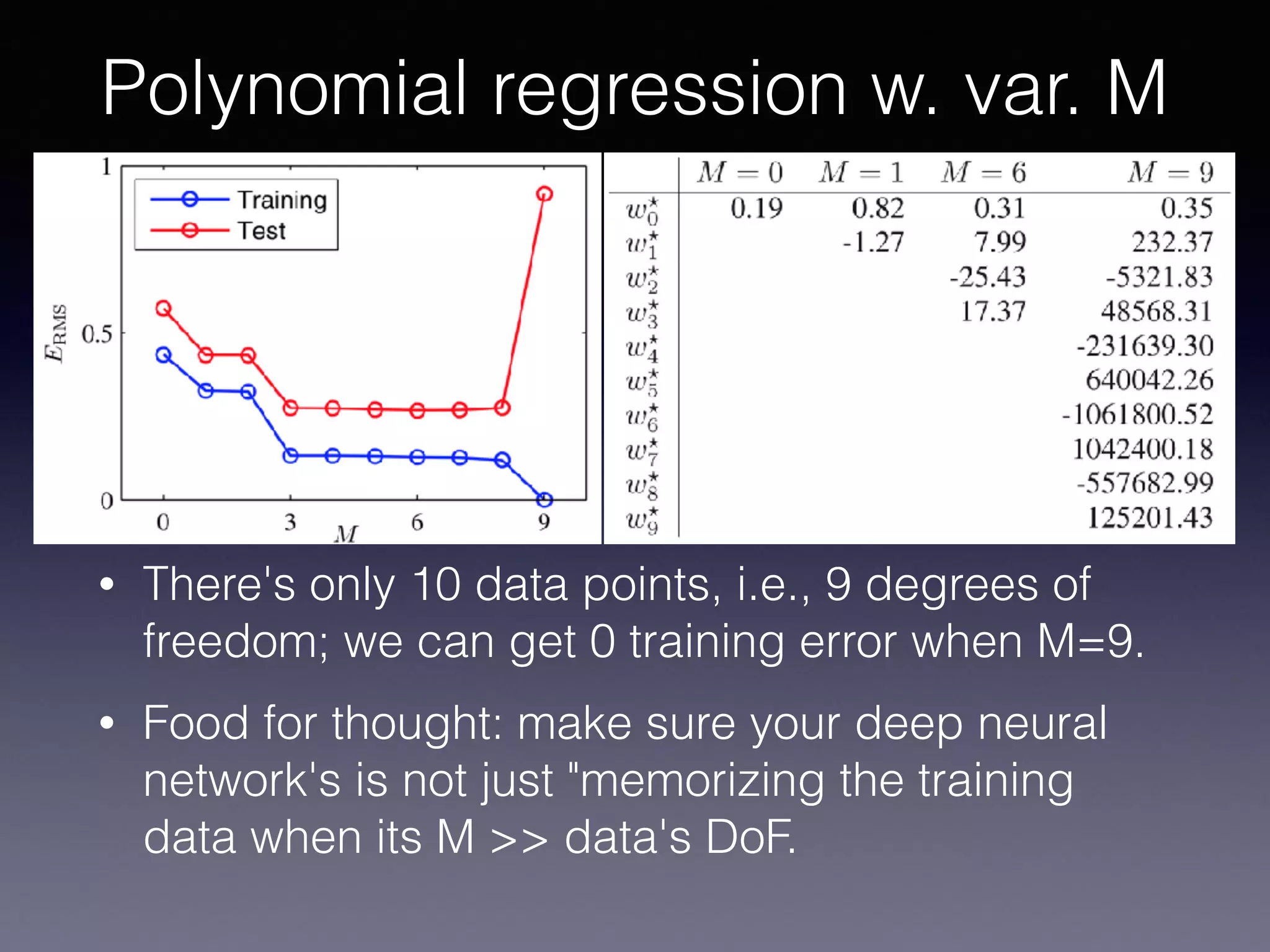
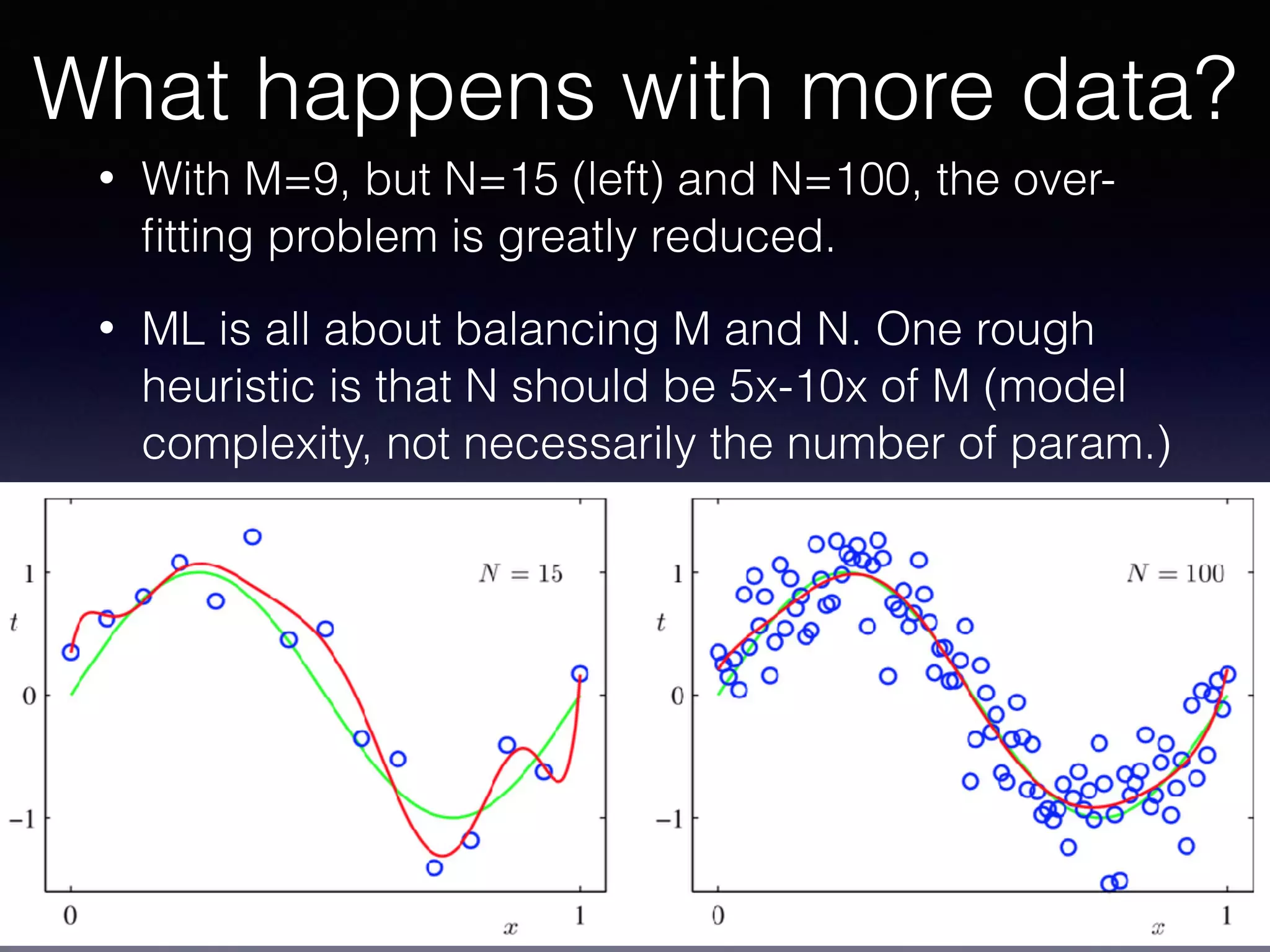
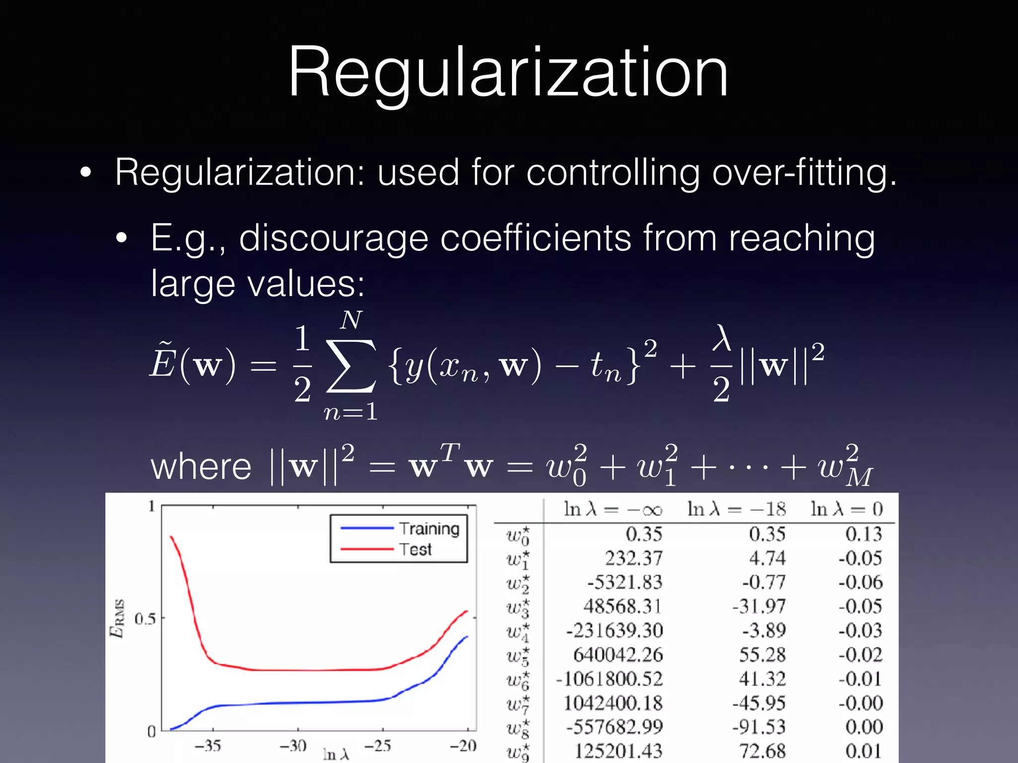
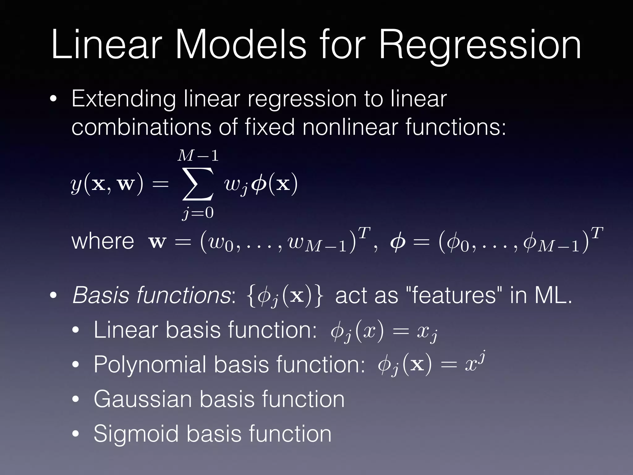
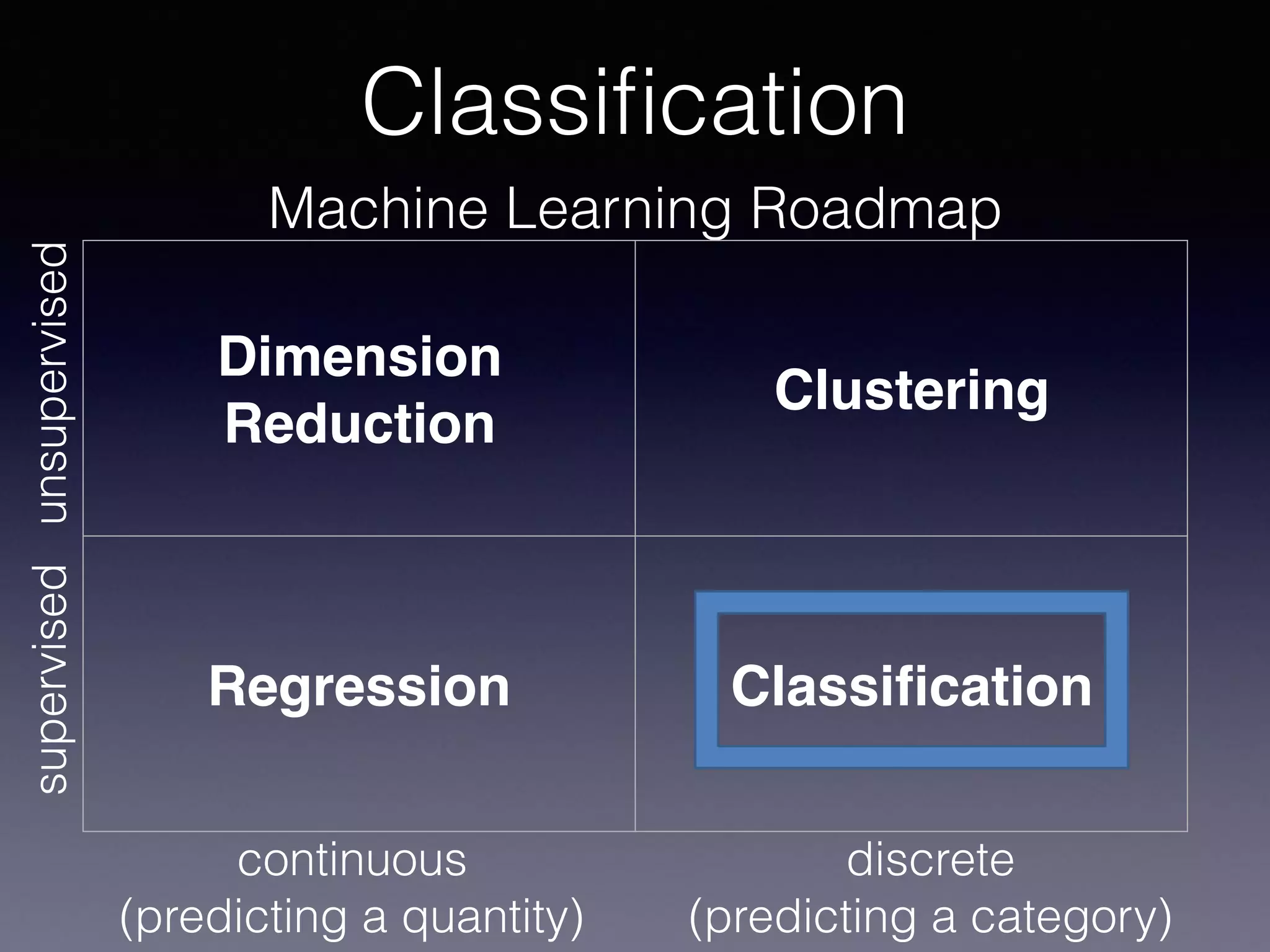


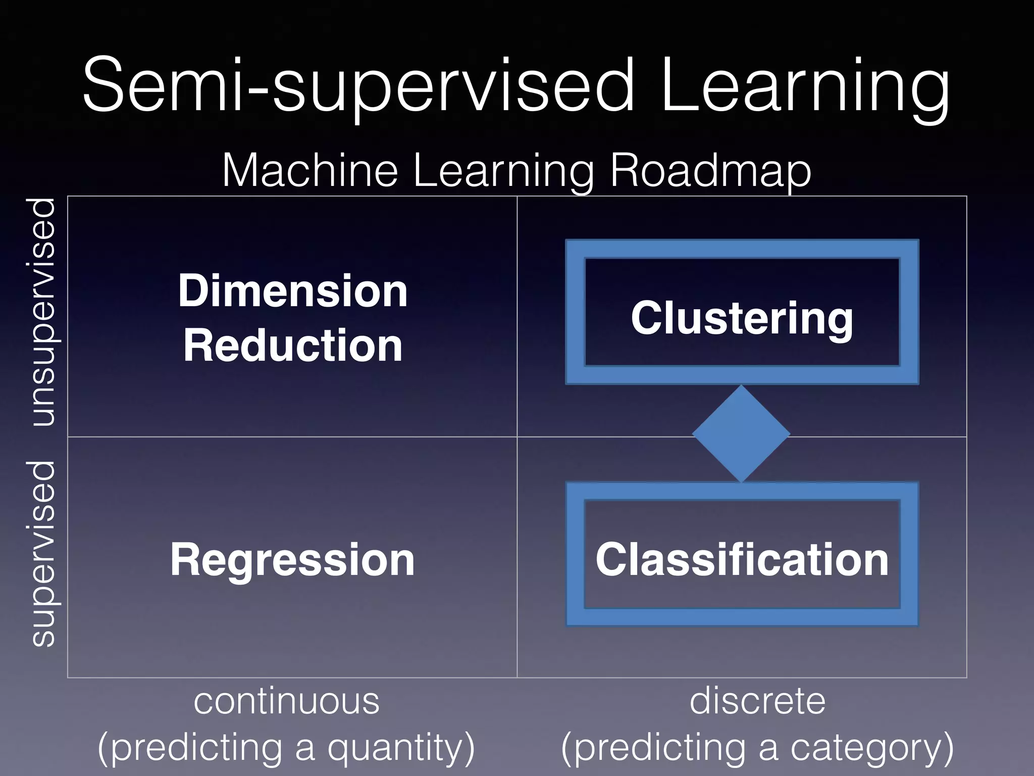

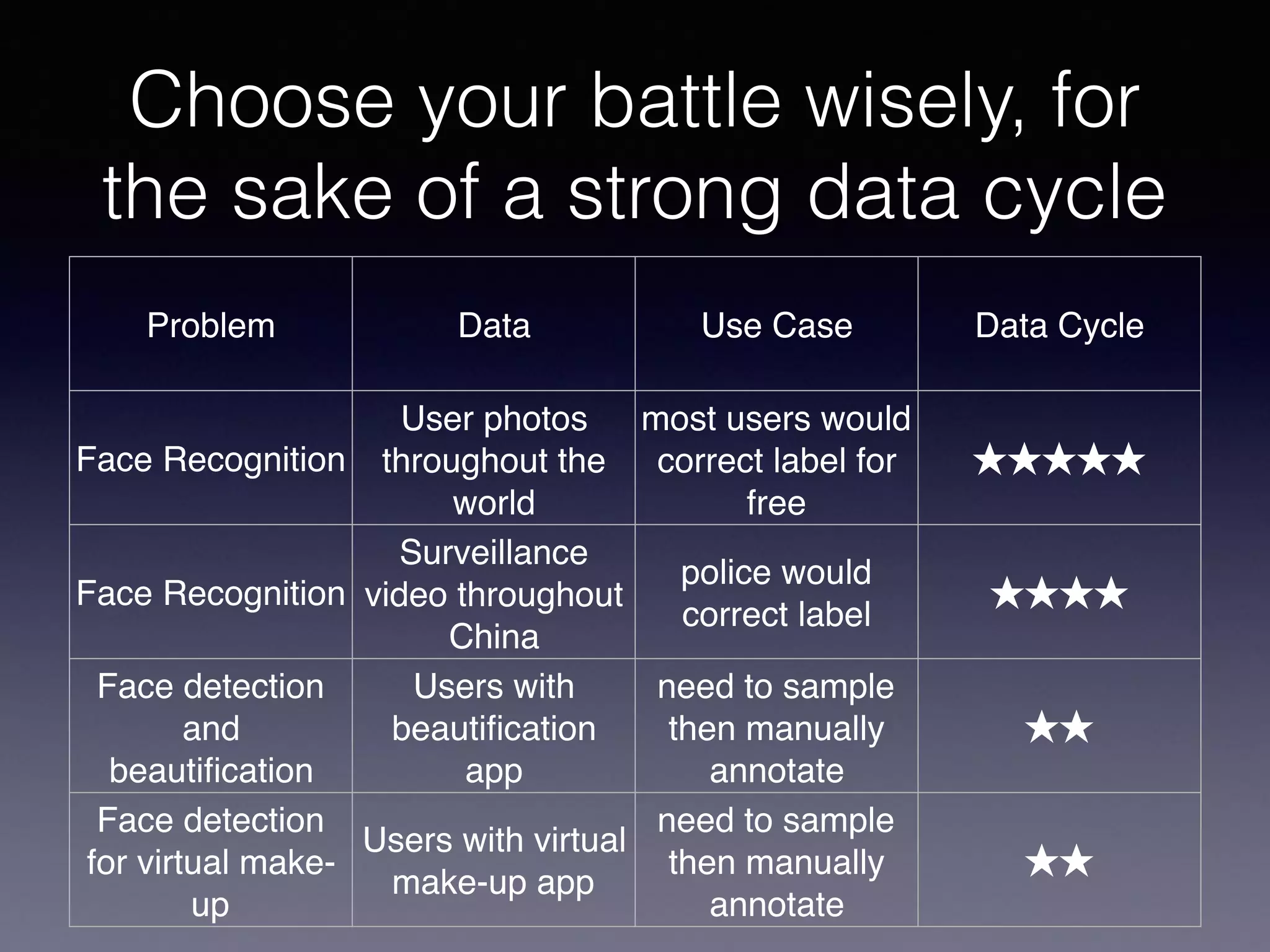


The document presents a comprehensive overview of machine learning foundations, including definitions and distinctions between manual programming and machine learning techniques. It discusses challenges such as the curse of dimensionality, differences in classification accuracy, and various ML approaches like dimension reduction, clustering, and regression. The document also details methods like PCA and GMM for data analysis, stressing the importance of feature selection and the impact of data volume and evolution on machine learning models.


![Vibe Coding vs. Spec-Driven Development [Free Meetup]](https://cdn.slidesharecdn.com/ss_thumbnails/vibecodingvsspecdrivendevelopment-251209105622-43f455e7-thumbnail.jpg?width=640&height=640&fit=bounds)
