MACHINE LEARNING UNIT 2

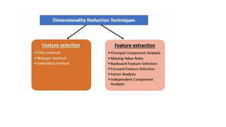
1. • Dimensionality Reduction: Principal Component Analysis, Singular
Value Decomposition.
• Nearest Neighbor Based Models: Introduction to Proximity Measures,
Distance Measures, Non-Metric Similarity Functions, Proximity
Between Binary Patterns, Different Classification Algorithms Based on
the Distance Measures, K-Nearest Neighbor Classifier, Radius Distance
Nearest Neighbor Algorithm, KNN Regression, Performance of
Classifiers.

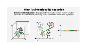
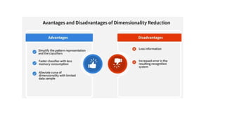
2. • When working with machine learning models, datasets with too many features can cause
issues like slow computation and overfitting.
• Dimensionality reduction helps to reduce the number of features while retaining key
information.
• Techniques like principal component analysis (PCA), singular value decomposition
(SVD) and linear discriminant analysis (LDA) convert data into a lower-dimensional space
while preserving important details.
Example: when you are building a model to predict house prices with features like bedrooms,
square footage and location. If you add too many features such as room condition or flooring
type, the dataset becomes large and complex.

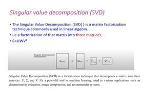
31. Singular Value Decomposition (SVD) is a factorization technique that decomposes a matrix into three
matrices: U, Σ, and V. It's a powerful tool in machine learning, used in various applications such as
dimensionality reduction, image compression, and recommender systems.

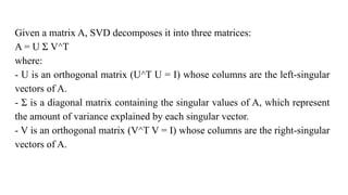
32. Given a matrix A, SVD decomposes it into three matrices:
A = U Σ V^T
where:
- U is an orthogonal matrix (U^T U = I) whose columns are the left-singular
vectors of A.
- Σ is a diagonal matrix containing the singular values of A, which represent
the amount of variance explained by each singular vector.
- V is an orthogonal matrix (V^T V = I) whose columns are the right-singular
vectors of A.

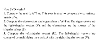
33. How SVD works?
1. Compute the matrix A^T A: This step is used to compute the covariance
matrix of A.
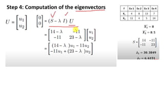
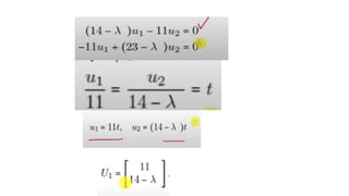
2. Compute the eigenvectors and eigenvalues of A^T A: The eigenvectors are
the right-singular vectors (V), and the eigenvalues are the squares of the
singular values (Σ).
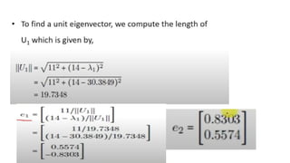
3. Compute the left-singular vectors (U): The left-singular vectors are
computed by multiplying the matrix A with the right-singular vectors (V).

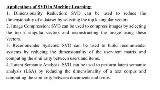
34. Applications of SVD in Machine Learning:
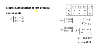
1. Dimensionality Reduction: SVD can be used to reduce the
dimensionality of a dataset by selecting the top k singular vectors.
2. Image Compression: SVD can be used to compress images by selecting
the top k singular vectors and reconstructing the image using these
vectors.
3. Recommender Systems: SVD can be used to build recommender
systems by reducing the dimensionality of the user-item matrix and
computing the similarity between users and items.
4. Latent Semantic Analysis: SVD can be used to perform latent semantic
analysis (LSA) by reducing the dimensionality of a text corpus and
computing the similarity between documents and terms.

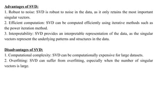
35. Advantages of SVD:
1. Robust to noise: SVD is robust to noise in the data, as it only retains the most important
singular vectors.
2. Efficient computation: SVD can be computed efficiently using iterative methods such as
the power iteration method.
3. Interpretability: SVD provides an interpretable representation of the data, as the singular
vectors represent the underlying patterns and structures in the data.
Disadvantages of SVD:
1. Computational complexity: SVD can be computationally expensive for large datasets.
2. Overfitting: SVD can suffer from overfitting, especially when the number of singular
vectors is large.

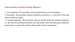
38. Characteristics of Good Proximity Measures:
1. Non-Negativity: The proximity measure should always be non-negative.
2. Symmetry: The proximity measure should be symmetric, i.e., the order of the data
points should not matter.
3. Triangle Inequality: The proximity measure should satisfy the triangle inequality,
i.e., the sum of the distances between two data points and a third data point should be
greater than or equal to the distance between the first two data points.

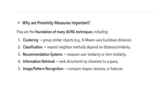
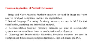
39. Common Applications of Proximity Measures:
1. Image and Video Analysis: Proximity measures are used in image and video
analysis for object recognition, tracking, and segmentation.
2. Natural Language Processing: Proximity measures are used in NLP for text
classification, clustering, and information retrieval.
3. Recommendation Systems: Proximity measures are used in recommender
systems to recommend items based on user behavior and preferences.
4. Clustering and Dimensionality Reduction: Proximity measures are used in
clustering and dimensionality reduction techniques, such as k-means and PCA.

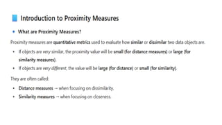
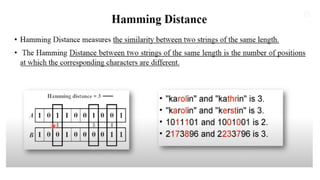
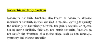
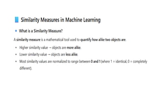
51. Non-metric similarity functions
Non-metric similarity functions, also known as non-metric distance
measures or similarity metrics, are used in machine learning to quantify
the similarity or dissimilarity between data points, features, or objects.
Unlike metric similarity functions, non-metric similarity functions do
not satisfy the properties of a metric space, such as non-negativity,
symmetry, and triangle inequality.

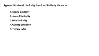
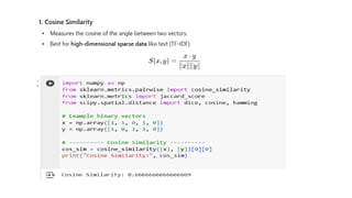
53. Types of Non-Metric Similarity Functions/Similarity Measures
1. Cosine Similarity
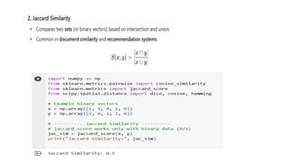
2. Jaccard Similarity
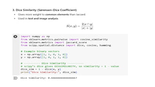
3. Dice Similarity
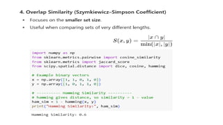
4. Overlap Similarity
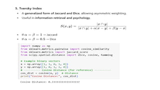
5. Tversky Index

61. Different Classification
Algorithms Based on the
Distance Measures

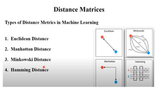
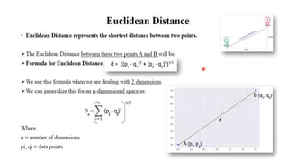
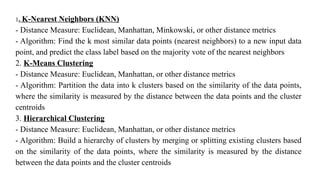
62. 1. K-Nearest Neighbors (KNN)
- Distance Measure: Euclidean, Manhattan, Minkowski, or other distance metrics
- Algorithm: Find the k most similar data points (nearest neighbors) to a new input data
point, and predict the class label based on the majority vote of the nearest neighbors
2. K-Means Clustering
- Distance Measure: Euclidean, Manhattan, or other distance metrics
- Algorithm: Partition the data into k clusters based on the similarity of the data points,
where the similarity is measured by the distance between the data points and the cluster
centroids
3. Hierarchical Clustering
- Distance Measure: Euclidean, Manhattan, or other distance metrics
- Algorithm: Build a hierarchy of clusters by merging or splitting existing clusters based
on the similarity of the data points, where the similarity is measured by the distance
between the data points and the cluster centroids

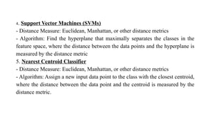
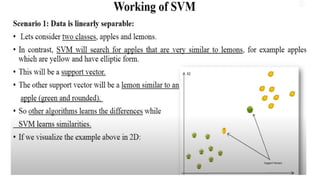
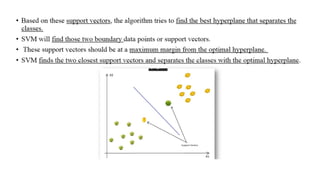
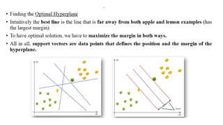
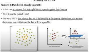
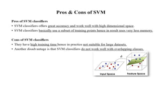
63. 4. Support Vector Machines (SVMs)
- Distance Measure: Euclidean, Manhattan, or other distance metrics
- Algorithm: Find the hyperplane that maximally separates the classes in the
feature space, where the distance between the data points and the hyperplane is
measured by the distance metric
5. Nearest Centroid Classifier
- Distance Measure: Euclidean, Manhattan, or other distance metrics
- Algorithm: Assign a new input data point to the class with the closest centroid,
where the distance between the data point and the centroid is measured by the
distance metric.

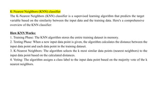
64. K-Nearest Neighbors (KNN) classifier
The K-Nearest Neighbors (KNN) classifier is a supervised learning algorithm that predicts the target
variable based on the similarity between the input data and the training data. Here's a comprehensive
overview of the KNN classifier:
How KNN Works:
1. Training Phase: The KNN algorithm stores the entire training dataset in memory.
2. Testing Phase: When a new input data point is given, the algorithm calculates the distance between the
input data point and each data point in the training dataset.
3. K-Nearest Neighbors: The algorithm selects the k most similar data points (nearest neighbors) to the
input data point based on the calculated distances.
4. Voting: The algorithm assigns a class label to the input data point based on the majority vote of the k
nearest neighbors.

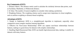
65. Key Components of KNN:
1. Distance Metric: The distance metric used to calculate the similarity between data points, such
as Euclidean, Manhattan, or Minkowski distance.
2. K-Value: The number of nearest neighbors to consider when making a prediction.
3. Weighting Scheme: The weighting scheme used to assign more importance to closer neighbors,
such as uniform weighting or distance-based weighting.
Advantages of KNN:
1. Simple to Implement: KNN is a straightforward algorithm to implement, especially when
compared to more complex machine learning algorithms.
2. Effective for Non-Linear Relationships: KNN can capture non-linear relationships between
features, making it a good choice for datasets with complex relationships.
3. Handling High-Dimensional Data: KNN can handle high-dimensional data, making it suitable for
datasets with many features.

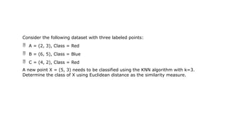
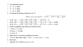
66. Consider the following dataset with three labeled points:
 A = (2, 3), Class = Red
 B = (6, 5), Class = Blue
 C = (4, 2), Class = Red
A new point X = (5, 3) needs to be classified using the KNN algorithm with k=3.
Determine the class of X using Euclidean distance as the similarity measure.

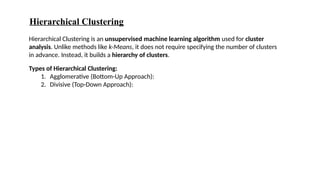
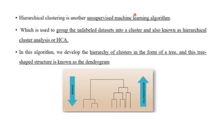
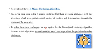
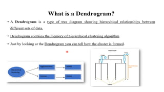
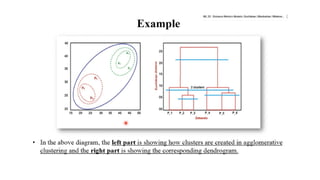
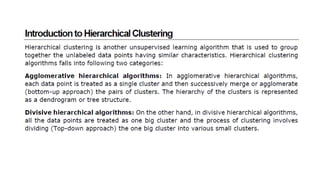
68. Hierarchical Clustering
Hierarchical Clustering is an unsupervised machine learning algorithm used for cluster
analysis. Unlike methods like k-Means, it does not require specifying the number of clusters
in advance. Instead, it builds a hierarchy of clusters.
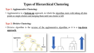
Types of Hierarchical Clustering:
1. Agglomerative (Bottom-Up Approach):
2. Divisive (Top-Down Approach):

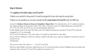
89. The Radius Distance Nearest Neighbor (RDNN) algorithm
The Radius Distance Nearest Neighbor (RDNN) algorithm is a
variation of the K-Nearest Neighbors (KNN) algorithm, which is used
for classification, regression, and other machine learning tasks. The
main difference between RDNN and KNN is that RDNN uses a radius-
based approach to find the nearest neighbors, whereas KNN uses a
fixed number of nearest neighbors (k).

90. How RDNN Works:
1. Training Phase: The RDNN algorithm stores the entire training dataset in memory.
2. Testing Phase: When a new input data point is given, the algorithm calculates the
distance between the input data point and each data point in the training dataset.
3. Radius-Based Search: The algorithm searches for all data points within a specified
radius (r) of the input data point.
4. Nearest Neighbors: The algorithm selects all data points within the radius (r) as the
nearest neighbors.
5. Voting: The algorithm assigns a class label to the input data point based on the
majority vote of the nearest neighbors.

91. Advantages of RDNN:
1. Flexibility: RDNN allows for a more flexible approach to finding nearest neighbors, as
the radius (r) can be adjusted based on the specific problem.
2. Robustness to Noise: RDNN can be more robust to noise and outliers in the data, as the
radius-based approach can help to filter out irrelevant data points.
3. Handling High-Dimensional Data: RDNN can handle high-dimensional data, making it
suitable for datasets with many features.

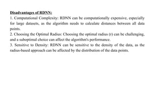
92. Disadvantages of RDNN:
1. Computational Complexity: RDNN can be computationally expensive, especially
for large datasets, as the algorithm needs to calculate distances between all data
points.
2. Choosing the Optimal Radius: Choosing the optimal radius (r) can be challenging,
and a suboptimal choice can affect the algorithm's performance.
3. Sensitive to Density: RDNN can be sensitive to the density of the data, as the
radius-based approach can be affected by the distribution of the data points.

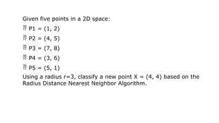
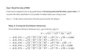
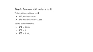
93. Given five points in a 2D space:
 P1 = (1, 2)
 P2 = (4, 5)
 P3 = (7, 8)
 P4 = (3, 6)
 P5 = (5, 1)
Using a radius r=3, classify a new point X = (4, 4) based on the
Radius Distance Nearest Neighbor Algorithm.

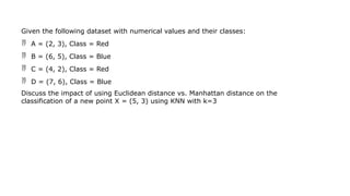
97. Given the following dataset with numerical values and their classes:
 A = (2, 3), Class = Red
 B = (6, 5), Class = Blue
 C = (4, 2), Class = Red
 D = (7, 6), Class = Blue
Discuss the impact of using Euclidean distance vs. Manhattan distance on the
classification of a new point X = (5, 3) using KNN with k=3

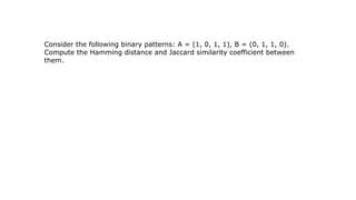
98. Consider the following binary patterns: A = (1, 0, 1, 1), B = (0, 1, 1, 0).
Compute the Hamming distance and Jaccard similarity coefficient between
them.

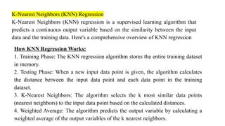
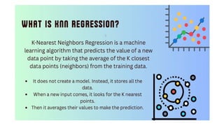
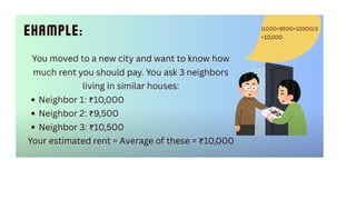
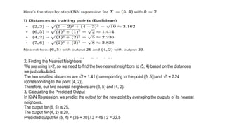
99. K-Nearest Neighbors (KNN) Regression
K-Nearest Neighbors (KNN) regression is a supervised learning algorithm that
predicts a continuous output variable based on the similarity between the input
data and the training data. Here's a comprehensive overview of KNN regression
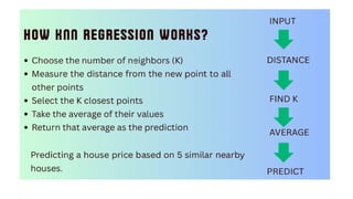
How KNN Regression Works:
1. Training Phase: The KNN regression algorithm stores the entire training dataset
in memory.
2. Testing Phase: When a new input data point is given, the algorithm calculates
the distance between the input data point and each data point in the training
dataset.
3. K-Nearest Neighbors: The algorithm selects the k most similar data points
(nearest neighbors) to the input data point based on the calculated distances.
4. Weighted Average: The algorithm predicts the output variable by calculating a
weighted average of the output variables of the k nearest neighbors.

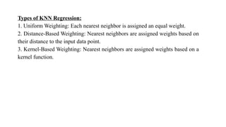
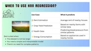
100. Types of KNN Regression:
1. Uniform Weighting: Each nearest neighbor is assigned an equal weight.
2. Distance-Based Weighting: Nearest neighbors are assigned weights based on
their distance to the input data point.
3. Kernel-Based Weighting: Nearest neighbors are assigned weights based on a
kernel function.

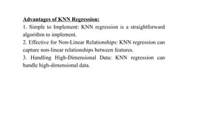
101. Advantages of KNN Regression:
1. Simple to Implement: KNN regression is a straightforward
algorithm to implement.
2. Effective for Non-Linear Relationships: KNN regression can
capture non-linear relationships between features.
3. Handling High-Dimensional Data: KNN regression can
handle high-dimensional data.

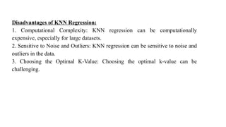
102. Disadvantages of KNN Regression:
1. Computational Complexity: KNN regression can be computationally
expensive, especially for large datasets.
2. Sensitive to Noise and Outliers: KNN regression can be sensitive to noise and
outliers in the data.
3. Choosing the Optimal K-Value: Choosing the optimal k-value can be
challenging.

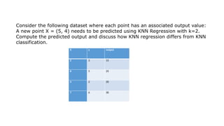
107. X y output
2 3 15
6 5 25
4 2 20
7 6 30
Consider the following dataset where each point has an associated output value:
A new point X = (5, 4) needs to be predicted using KNN Regression with k=2.
Compute the predicted output and discuss how KNN regression differs from KNN
classification.

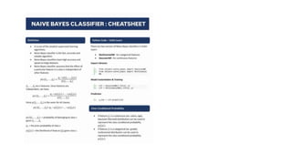
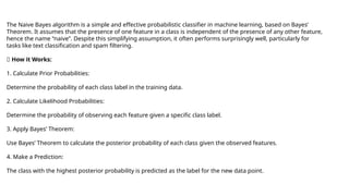
112. The Naive Bayes algorithm is a simple and effective probabilistic classifier in machine learning, based on Bayes’
Theorem. It assumes that the presence of one feature in a class is independent of the presence of any other feature,
hence the name “naive”. Despite this simplifying assumption, it often performs surprisingly well, particularly for
tasks like text classification and spam filtering.
✅ How it Works:
1. Calculate Prior Probabilities:
Determine the probability of each class label in the training data.
2. Calculate Likelihood Probabilities:
Determine the probability of observing each feature given a specific class label.
3. Apply Bayes’ Theorem:
Use Bayes’ Theorem to calculate the posterior probability of each class given the observed features.
4. Make a Prediction:
The class with the highest posterior probability is predicted as the label for the new data point.

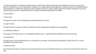
113. ✅ Logistic regression is a statistical method used in machine learning for predicting the probability of a binary outcome (e.g.,
yes/no, 0/1) based on a set of independent variables. It’s a supervised learning algorithm, meaning it learns from labeled data to
make predictions. Unlike linear regression which predicts continuous values, logistic regression predicts categorical outcomes,
using the logit function (or sigmoid function) to model the relationship between variables.
✅ How it Works:
1. Data Input:
The algorithm takes a set of independent variables (features) as input.
2. Logit Function:
The logit function transforms a linear combination of the independent variables into a probability.
3. Probability Prediction:
The output of the logit function is a probability between 0 and 1, representing the likelihood of the positive class.
4. Classification:
The data point is then classified based on a threshold. For example, if the predicted probability is greater than 0.5, it can be
classified as the positive class.
5. Model Training:
The model’s parameters are learned using techniques like maximum likelihood estimation, which aims to find the best fit for the
data.

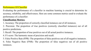
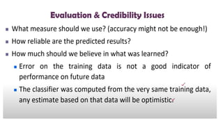
115. Performance Of Classifier
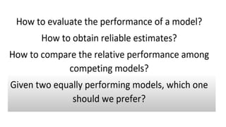
Evaluating the performance of a classifier in machine learning is crucial to determine its
accuracy, reliability, and effectiveness. Here are some common metrics used to evaluate the
performance of a classifier:
Classification Metrics:
1. Accuracy: The proportion of correctly classified instances out of all instances.
2. Precision: The proportion of true positives (correctly classified instances) out of all
positive predictions.
3. Recall: The proportion of true positives out of all actual positive instances.
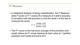
4. F1-score: The harmonic mean of precision and recall.
5. False Positive Rate (FPR): The proportion of false positives out of all negative instances.
6. False Negative Rate (FNR): The proportion of false negatives out of all positive
instances.

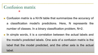
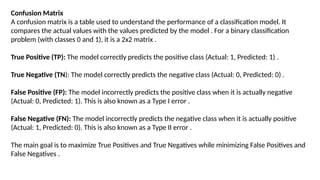
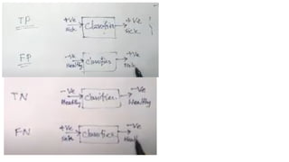
131. Confusion Matrix
A confusion matrix is a table used to understand the performance of a classification model. It
compares the actual values with the values predicted by the model . For a binary classification
problem (with classes 0 and 1), it is a 2x2 matrix .
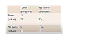
True Positive (TP): The model correctly predicts the positive class (Actual: 1, Predicted: 1) .
True Negative (TN): The model correctly predicts the negative class (Actual: 0, Predicted: 0) .
False Positive (FP): The model incorrectly predicts the positive class when it is actually negative
(Actual: 0, Predicted: 1). This is also known as a Type I error .
False Negative (FN): The model incorrectly predicts the negative class when it is actually positive
(Actual: 1, Predicted: 0). This is also known as a Type II error .
The main goal is to maximize True Positives and True Negatives while minimizing False Positives and
False Negatives .

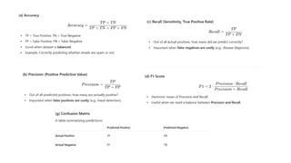
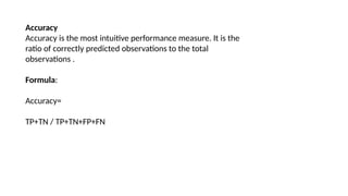
132. Accuracy
Accuracy is the most intuitive performance measure. It is the
ratio of correctly predicted observations to the total
observations .
Formula:
Accuracy=
TP+TN / TP+TN+FP+FN

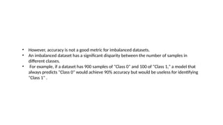
133. • However, accuracy is not a good metric for imbalanced datasets.
• An imbalanced dataset has a significant disparity between the number of samples in
different classes.
• For example, if a dataset has 900 samples of "Class 0" and 100 of "Class 1," a model that
always predicts "Class 0" would achieve 90% accuracy but would be useless for identifying
"Class 1" .

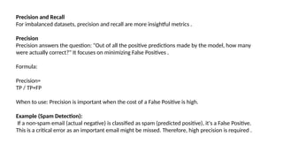
134. Precision and Recall
For imbalanced datasets, precision and recall are more insightful metrics .
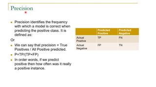
Precision
Precision answers the question: "Out of all the positive predictions made by the model, how many
were actually correct?" It focuses on minimizing False Positives .
Formula:
Precision=
TP / TP+FP
When to use: Precision is important when the cost of a False Positive is high.
Example (Spam Detection):
If a non-spam email (actual negative) is classified as spam (predicted positive), it's a False Positive.
This is a critical error as an important email might be missed. Therefore, high precision is required .

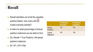
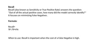
135. Recall
Recall (also known as Sensitivity or True Positive Rate) answers the question:
"Out of all the actual positive cases, how many did the model correctly identify?"
It focuses on minimizing False Negatives .
Formula:
Recall=
TP /TP+FN
When to use: Recall is important when the cost of a False Negative is high.

136. Recall is more important (
β
β > 1): A value like
β
β = 2 is used. This gives more weight to recall, which is critical for problems like cancer diagnosis .
Choosing the correct metric often requires domain expertise to understand the relative importance of minimizing False
Positives versus False Negatives for a specific application

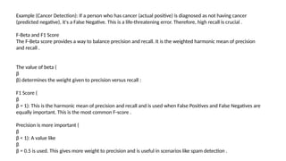
137. Example (Cancer Detection): If a person who has cancer (actual positive) is diagnosed as not having cancer
(predicted negative), it's a False Negative. This is a life-threatening error. Therefore, high recall is crucial .
F-Beta and F1 Score
The F-Beta score provides a way to balance precision and recall. It is the weighted harmonic mean of precision
and recall .
The value of beta (
β
β) determines the weight given to precision versus recall :
F1 Score (
β
β = 1): This is the harmonic mean of precision and recall and is used when False Positives and False Negatives are
equally important. This is the most common F-score .
Precision is more important (
β
β < 1): A value like
β
β = 0.5 is used. This gives more weight to precision and is useful in scenarios like spam detection .