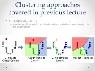
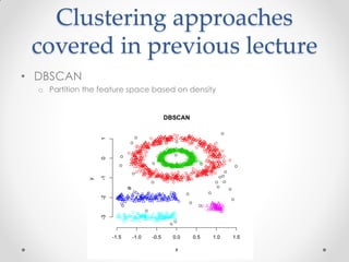
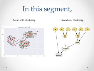
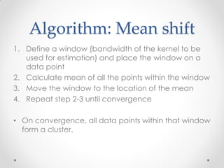
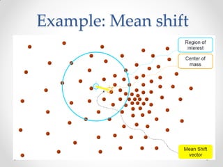
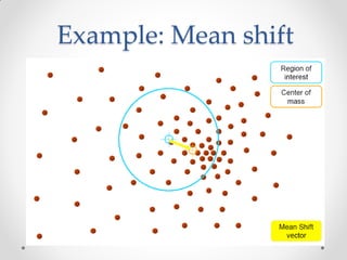
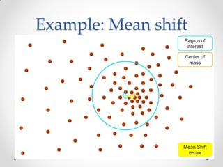
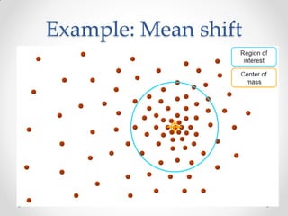
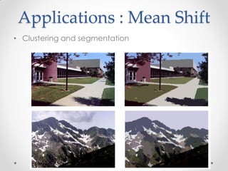
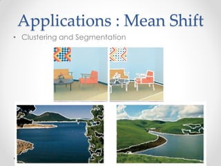
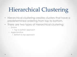
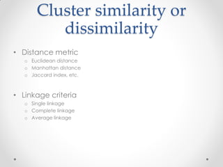
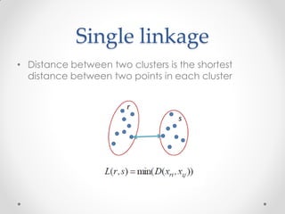
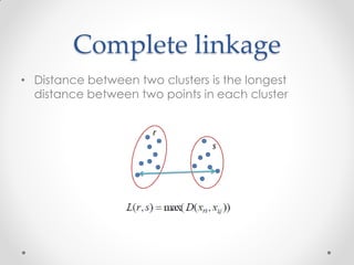
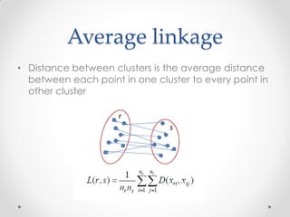
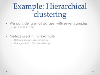
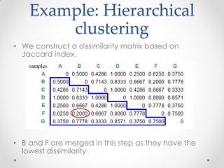
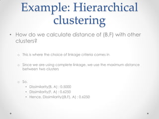
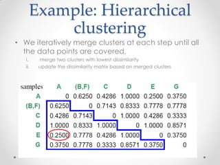
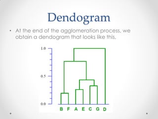
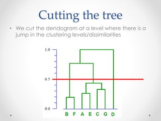
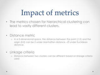
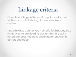
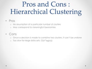
Mean shift clustering finds clusters by locating peaks in the probability density function of the data. It iteratively moves data points to the mean of nearby points until convergence. Hierarchical clustering builds clusters gradually by either merging or splitting clusters at each step. There are two types: divisive which splits clusters, and agglomerative which merges clusters. Agglomerative clustering starts with each point as a cluster and iteratively merges the closest pair of clusters until all are merged based on a chosen linkage method like complete or average linkage. The choice of distance metric and linkage method impacts the resulting clusters.

1. Clustering for new discovery in data
Mean shift clustering
Hierarchical clustering
- Kunal Parmar
Houston Machine
Learning Meetup
1/21/2017

2. Clustering : A world
without labels
• Finding hidden structure in data when we don’t
have labels/classes for the data
• We group data
together based
on some notion
of similarity in
the feature space

3. Clustering approaches
covered in previous lecture
• k-means clustering
o Iterative partitioning into k clusters based on proximity of an observation to
the cluster mean

4. Clustering approaches
covered in previous lecture
• DBSCAN
o Partition the feature space based on density

5. In this segment,
Mean shift clustering Hierarchical clustering

6. Mean shift clustering
• Mean shift clustering is a non-parametric iterative
mode-based clustering technique based on kernel
density estimation.
• It is very commonly used in the field of computer
vision because of it’s high efficiency in image
segmentation.

7. Mean shift clustering
• It assumes that our data is sampled from an
underlying probability distribution
• The algorithm finds out the modes(peaks) of the
probability distribution. The underlying kernel
distribution at the mode corresponds to a cluster

8. Kernel density estimation
Set of points KDE surface

9. Algorithm: Mean shift
1. Define a window (bandwidth of the kernel to be
used for estimation) and place the window on a
data point
2. Calculate mean of all the points within the window
3. Move the window to the location of the mean
4. Repeat step 2-3 until convergence
• On convergence, all data points within that window
form a cluster.

10. Example: Mean shift

11. Example: Mean shift

12. Example: Mean shift

13. Example: Mean shift

14. Types of kernels
• Generally, a Gaussian kernel is used for probability
estimation in mean shift clustering.
• However, other kinds of kernels that can be used
are,
o Rectangular kernel
o Flat kernel, etc.
• The choice of kernel affects the clustering result

15. Types of kernels
• The choice of the bandwidth of the kernel(window)
will also impact the clustering result
o Small kernels will result in lots of clusters, some even being individual data
points
o Big kernels will result in one or two huge clusters

16. Pros and cons : Mean Shift
• Pros
o Model-free, doesn’t assume predefined shape of clusters
o Only relies on one parameter: kernel bandwidth h
o Robust to outliers
• Cons
o The selection of window size is not trivial
o Computationally expensive; O(𝑛2
)
o Sensitive to selection of kernel bandwidth; small h will slow down convergence,
large h speeds it up but might merge two modes

17. Applications : Mean Shift
• Clustering and segmentation
• dfsn

18. Applications : Mean Shift
• Clustering and Segmentation

19. Hierarchical Clustering
• Hierarchical clustering creates clusters that have a
predetermined ordering from top to bottom.
• There are two types of hierarchical clustering:
o Divisive
• Top to bottom approach
o Agglomerative
• Bottom to top approach

20. Algorithm:
Hierarchical agglomerative clustering
1. Place each data point in it’s own singleton group
2. Iteratively merge the two closest groups
3. Repeat step 2 until all the data points are merged
into a single cluster
• We obtain a dendogram(tree-like structure) at the
final step. We cut the dendogram at a certain level
to obtain the final set of clusters.

21. Cluster similarity or
dissimilarity
• Distance metric
o Euclidean distance
o Manhattan distance
o Jaccard index, etc.
• Linkage criteria
o Single linkage
o Complete linkage
o Average linkage

22. Linkage criteria
• It is the quantification of the distance between sets
of observations/intermediate clusters formed in the
agglomeration process

23. Single linkage
• Distance between two clusters is the shortest
distance between two points in each cluster

24. Complete linkage
• Distance between two clusters is the longest
distance between two points in each cluster

25. Average linkage
• Distance between clusters is the average distance
between each point in one cluster to every point in
other cluster

26. Example: Hierarchical
clustering
• We consider a small dataset with seven samples;
o (A, B, C, D, E, F, G)
• Metrics used in this example
o Distance metric: Jaccard index
o Linkage criteria: Complete linkage

27. Example: Hierarchical
clustering
• We construct a dissimilarity matrix based on
Jaccard index.
• B and F are merged in this step as they have the
lowest dissimilarity

28. Example: Hierarchical
clustering
• How do we calculate distance of (B,F) with other
clusters?
o This is where the choice of linkage criteria comes in
o Since we are using complete linkage, we use the maximum distance
between two clusters
o So,
• Dissimilarity(B, A) : 0.5000
• Dissimilarity(F, A) : 0.6250
• Hence, Dissimilarity((B,F), A) : 0.6250

29. Example: Hierarchical
clustering
• We iteratively merge clusters at each step until all
the data points are covered,
i. merge two clusters with lowest dissimilarity
ii. update the dissimilarity matrix based on merged clusters
o sfs

30. Dendogram
• At the end of the agglomeration process, we
obtain a dendogram that looks like this,
• sfdafdfsdfsd

31. Cutting the tree
• We cut the dendogram at a level where there is a
jump in the clustering levels/dissimilarities

32. Cutting the tree
• If we cut the tree at 0.5, then we can say that within
each cluster the samples have more than 50%
similarity
• So our final set of clusters is,
i. (B,F),
ii. (A,E,C,G) and
iii. (D)

33. Final set of clusters

34. Impact of metrics
• The metrics chosen for hierarchical clustering can
lead to vastly different clusters.
• Distance metric
o In a 2-dimensional space, the distance between the point (1,0) and the
origin (0,0) can be 2 under Manhattan distance, 2 under Euclidean
distance.
• Linkage criteria
o Distance between two clusters can be different based on linkage criteria
used

35. Linkage criteria
• Complete linkage is the most popular metric used
for hierarchical clustering. It is less sensitive to
outliers.
• Single linkage can handle non-elliptical shapes. But,
single linkage can lead to clusters that are quite
heterogeneous internally and it more sensitive to
outliers and noise

36. Pros and Cons :
Hierarchical Clustering
• Pros
o No assumption of a particular number of clusters
o May correspond to meaningful taxonomies
• Cons
o Once a decision is made to combine two clusters, it can’t be undone
o Too slow for large data sets, O(𝑛2
log(𝑛))

37. References
i. https://spin.atomicobject.com/2015/05/26/mean-
shift-clustering/
ii. http://vision.stanford.edu/teaching/cs131_fall1314
_nope/lectures/lecture13_kmeans_cs131.pdf
iii. http://84.89.132.1/~michael/stanford/maeb7.pdf

38. Thank you!