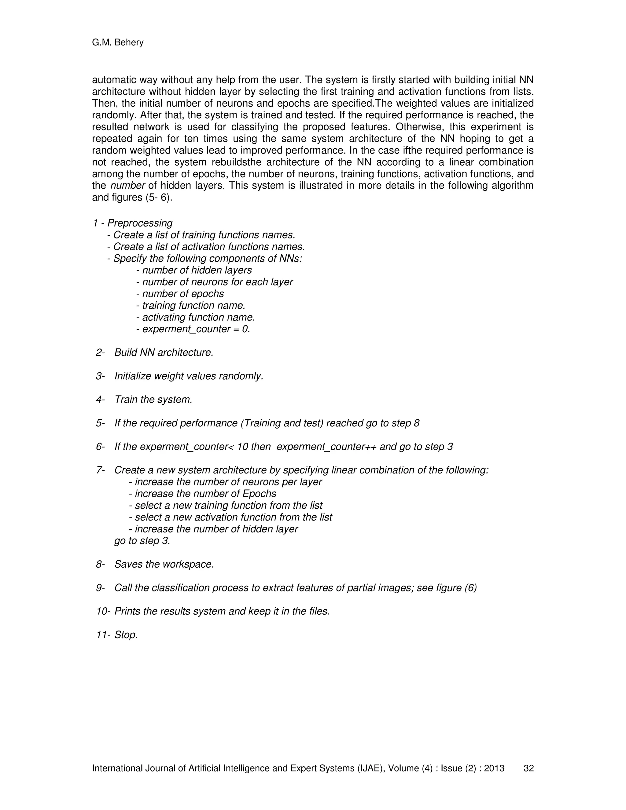
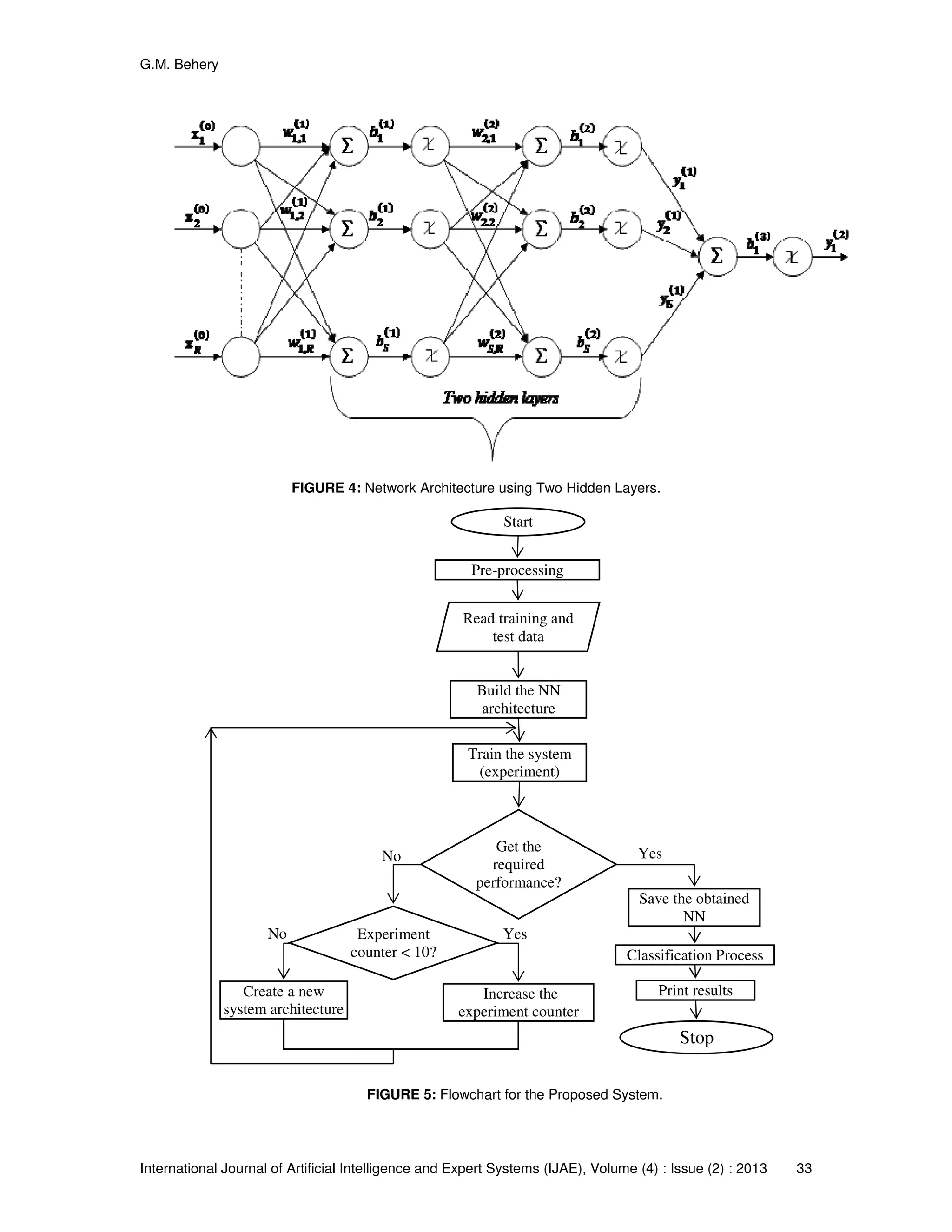
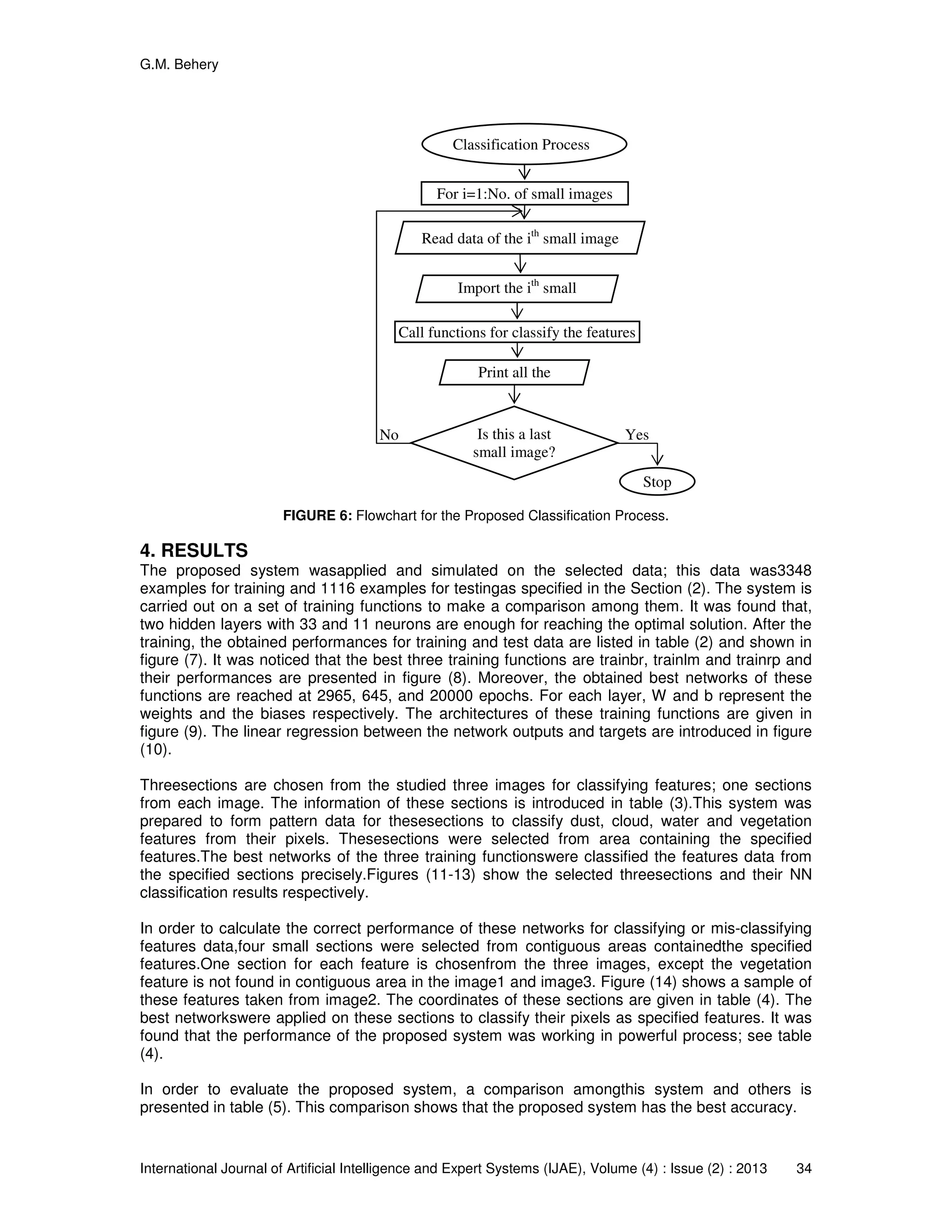
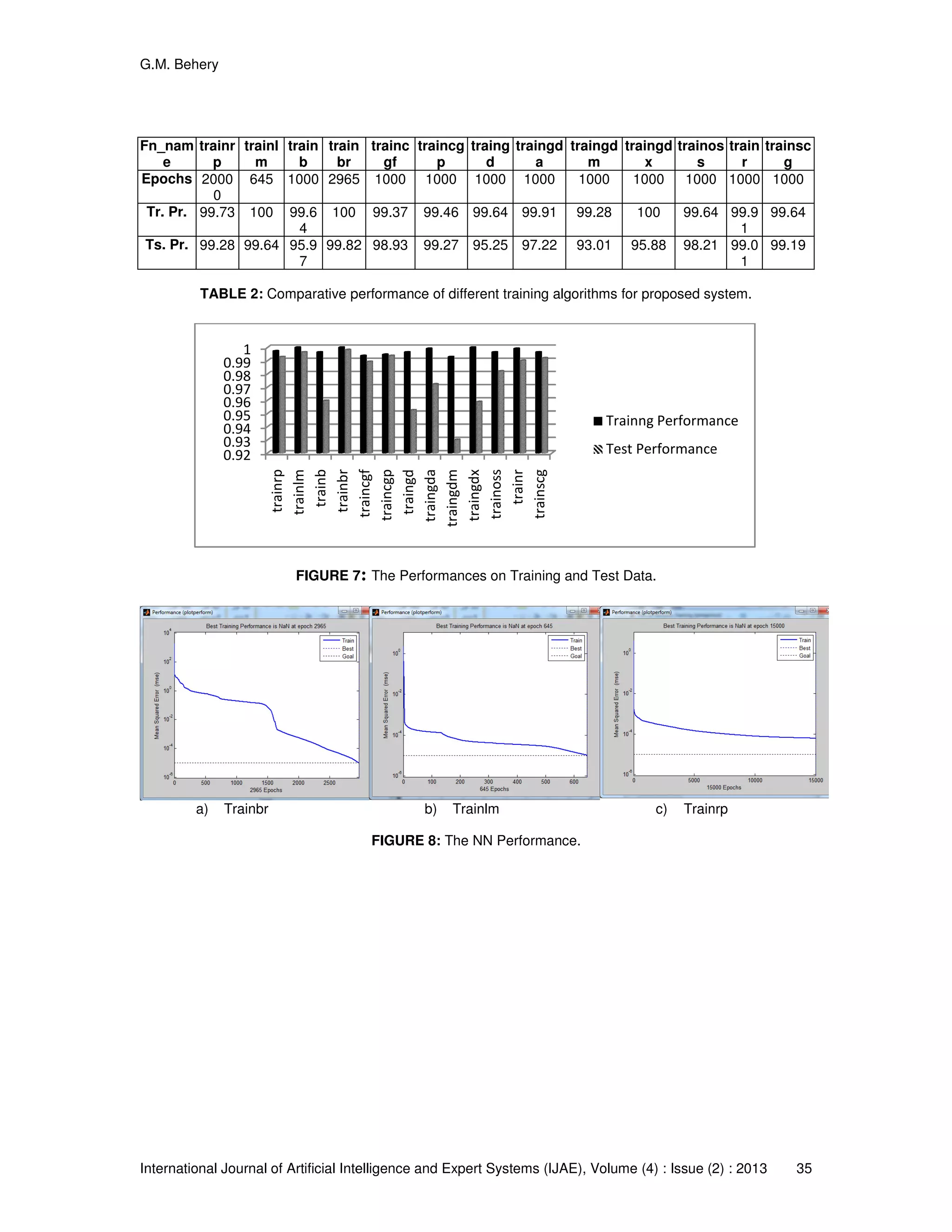
An Automatic Neural Networks System for Classifying Dust, Clouds, Water, and Vegetation from Red Sea Area

G.M. Behery
International Journal of Artificial Intelligence and Expert Systems (IJAE), Volume (4) : Issue (2) : 2013 27
An Automatic Neural Networks System for Classifying Dust,
Clouds, Water, and Vegetation from Red Sea Area
G.M. Behery behery2911961@yahoo.com
Faculty of science, Math.and Comp. Department
Damietta University
New Damietta, 34517, Egypt.
Abstract
This paper presents an automatic remotely sensed system that is designed to classify dust,
clouds, water and vegetation features from red sea area. Thus provides the system to make the
test and classification process without retraining again. This system can rebuild the architecture
of the neural network (NN) according to a linear combination among the number of epochs, the
number of neurons, training functions, activation functions, and the number of hidden layers.
Theproposed system is trained on the features of the provided images using 13 training functions,
and is designed to find the best networks that has the ability to have the best classification on
data is not included in the training data.This system shows an excellent classification of test data
that is collected from the training data. The performances of the best three training
functionsare%99.82, %99.64 and %99.28for test data that is not included in the training
data.Although, the proposed system was trained on data selected only from one image, this
system shows correctly classification of the features in the all images. The designed system can
be carried out on remotely sensed images for classifying other features.This system was applied
on several sub-images to classify the specified features. The correct performance of classifying
the features from the sub-images was calculated by applying the proposed system on some small
sections that were selected from contiguous areas contained the features.
Keywords: NNs , Image Processing, Classification, Dust, Clouds, Water, Vegetation.
1. INTRODUCTION
Remote sensing images provide a general reflection of the spatial characteristics for ground
objects. Extraction of land-cover map information from multispectral or hyperspectral remotely
sensed images is one of the important tasks of remote sensing technology [1-3]. Precise
information about the landuse and land cover changes of the Earth’s surface is extremely
important for any kind of sustainable development program [4, 5].In order to automatically
generate such landuse map from remotely sensed images, various pattern recognition techniques
like classification and clustering can be adopted [6, 7]. These images are used in many
applications e.g. for detecting the change in ground cover [8-10], extraction of forest [11-13], and
many others [14-16].
NN algorithms are widely used for classifying features from remotely sensed images [17, 18].NN
offers a number of advantages over conventional statistical classifiers such as the maximum
likelihood classifier. Perhaps the most important characteristic of NN is that there is no underlying
assumption about the distribution of data. Furthermore, it is easy to use data from different
sources in the NN classification procedure to improve the accuracy of the classification. NN
algorithms have some handicaps related in particular to the long training time requirement and
finding the most efficient network structure. Large networks take a long time to learn the data
whilst small networks may become trapped into a local minimum and may not learn from the
training data. The structure of the network has a direct effect on training time and classification
accuracy. The NN architecture which gives the best result for a particular problem can only be
determined experimentally. Unfortunately, there is currently no available direct method developed

G.M. Behery
for this purpose [19, 20]. The NN algorithms are always iterative, designed to step by step
minimise the difference between the actual output vector of the network and the desired output
vector. The Backpropagation (BP) algorithm is effective method for classifying features from
images [21, 22].
The following training functions are chosen as classifiers in the proposed system. They are
Resilient Propagation (trainrp) [23, 26, 34-37], Gradient descent (traingd) [38], Gradient descent
with momentum (traingdm) [38], Scaled conjugate gradient (trainscg) [39], Levenberg-Marquardt
(trainlm) [40], Random order incremental training with learning functions (trainr) [41], Bayesian
regularization (trainbr) [41], One step secant (trainoss) [42], Gradient descent with momentumand
adaptive learning rule (traingdx) [43-44], Gradient descent with adaptive learning rule (traingda)
[45], Fletcher-Powell conjugate gradient (traincgf) [38, 46], Polak-Ribiére conjugate gradient
(traincgp)[46], and Batch training with weight and bias learning rules (trainb)[47] backpropagation
algorithms.
This work is usedNN for classifying dust, clouds, water and vegetation features from red sea
area. BP is the most widely used algorithm for supervised learning with multi-layered feed-
forward networks and it is very well known, while the trainrpfunction is not well known. The
trainrpfunctionis faster than all the other BP functions[27-30]. The rest of paper is organized as
follows; Section 2 describes the pattern data that is used for training and testing the system.
Section 3 presents the proposed system. Section 4 shows the obtained results. Finally, Section5
concludes the work.
2. PATTERN DATA
This study is carried out on three images that were obtained by the Moderate Resolution Imaging
Spectroradiometer(MODIS) on NASA’s Aqua satellite. The first image contains multiple dust
plumes blew eastward across the Red Sea. Along the eastern edge of the Red Sea, some of the
dust forms wave patterns. Over the Arabian Peninsula, clouds fringe the eastern edge of a giant
veil of dust. East of the clouds, skies are clear. Along the African coast, some of the smaller,
linear plumes in the south may have arisen from sediments near the shore, especially the plumes
originating in southern Sudan. The wide, opaque plume in the north, however, may have arisen
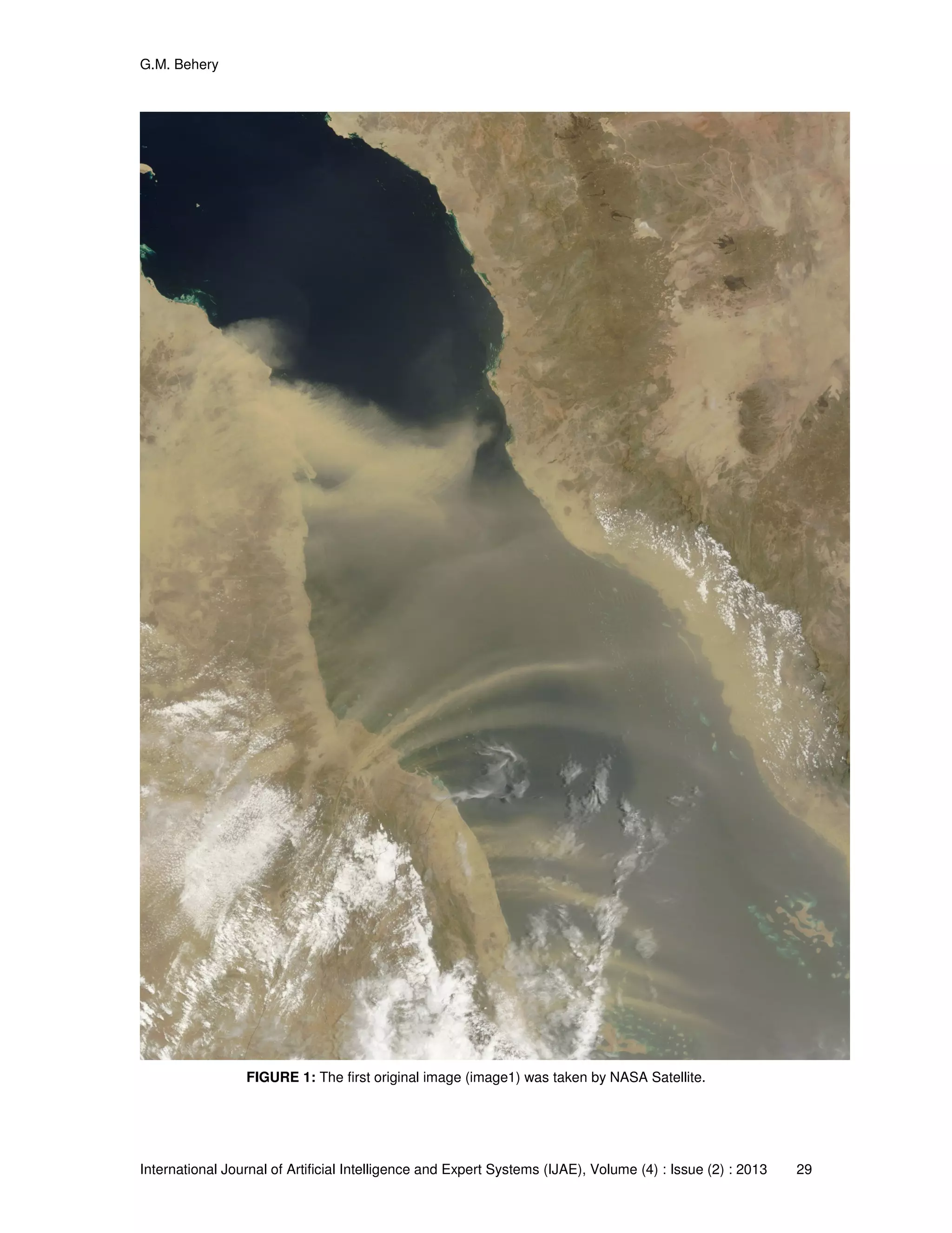
farther inland, perhaps from sand seas in the Sahara [31]; see figure(1). The second one has
dust plumes blew off the coast of Africa and over the Red Sea. The dust blowing off the coast of
Sudan is thick enough to completely hide the land and water surface below, but the thickest dust
stops short of reaching Saudi Arabia. Farther south, between Eritrea and Yemen, a thin dusty
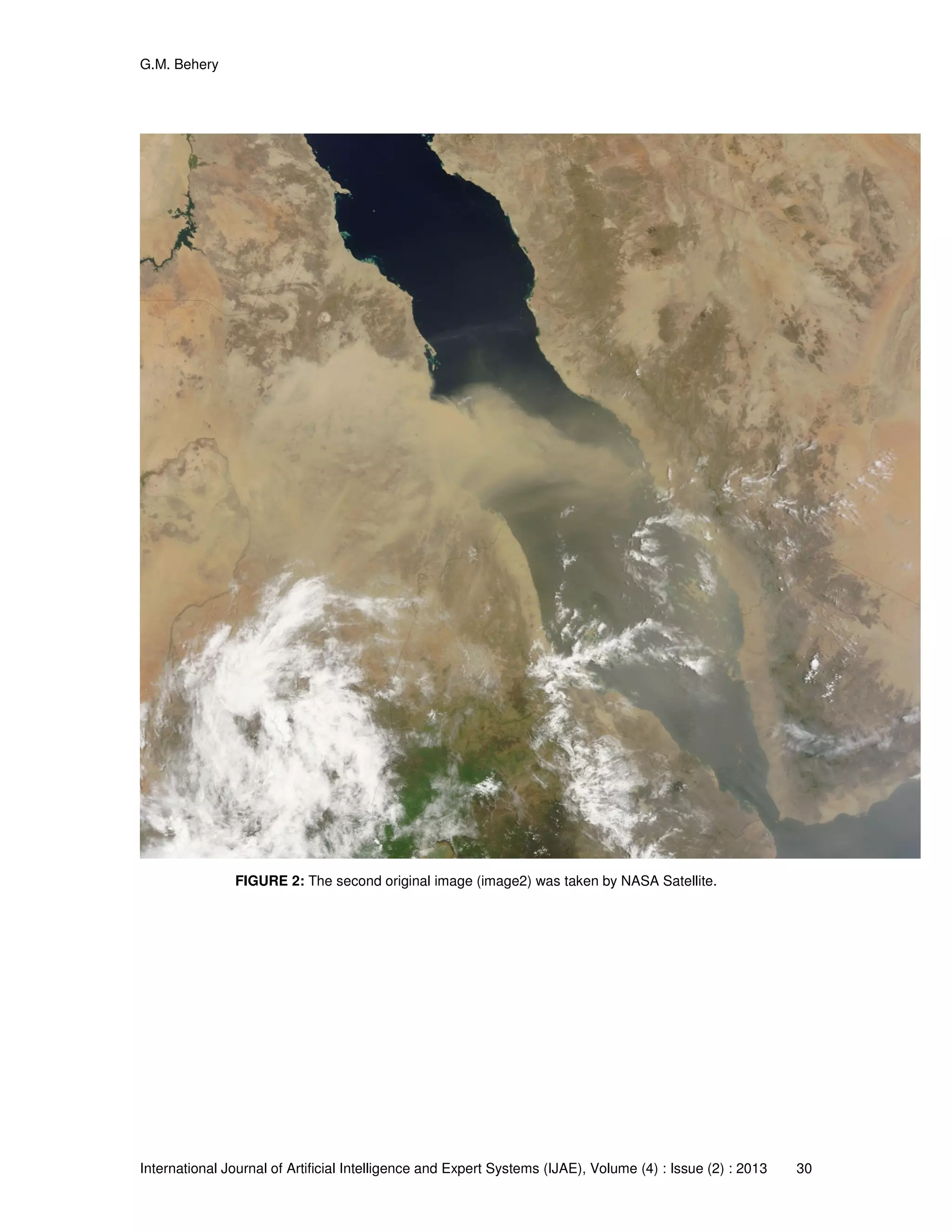
haze hangs over the Red Sea [32]; see figure (2). The third contains dust plumes blew off the
coast of Sudan and across the Red Sea. Two distinct plumes arise not far from the coast of
Sudan and blow toward the northeast. The northern plume almost reaches Saudi Arabia. North of
these plumes, a veil of dust with indistinct margins extends from Sudan most of the way across
the water [33]; see figure (3). These three images are called image1, image2, and image3
respectively. They are RGB format and their information is shown in table (1).
In this study, the classification is specified for dust, clouds, water, and vegetation features. Each
feature has approximately the same colour in the three images. So, the pattern data is selected
randomly by sampling throughout the image2 only. Where, it contains all features clearly. The
selection of this data is such that it contains samples of all features. The pattern data for each
pixel consists of three pixel grey-levels, one for each band. These bands are red, green and blue.
The grey levels in the original images are coded as eight bits binary numbers in the range from 0
to 255. In order to train the NNs, all pixels values are normalised to lie between 0.0 and 1.0. The
pattern data is collected from the proposed image for the features: dust, clouds, water, and
vegetation. After the collection, each feature is represented as one group. Each group is divided
into two parts: two-thirds for training and one third for test. Then, the training groups are merged
in single file, and the test groups in other file.

G.M. Behery
FIGURE 1: The first original image (image1) was taken by NASA Satellite.

G.M. Behery
FIGURE 2: The second original image (image2) was taken by NASA Satellite.

G.M. Behery
FIGURE 3: The third original image (image3) was taken by NASA Satellite.
Name taken date length width size /MB
image1 July 24, 2010 4000 2800 1.14
image2 mid-July 2011 5916 6372 3.14
image3 Aug. 3, 2011 5916 6372 3.25
TABLE 1: Information of the Studied Three Images.
3. PROPOSED SYSTEM
NNsare very effective methods to classify features fromimages. Figure (4)shows the NN
architecture. This architectureconsists of input layer with R elements, two hidden layers with S
neurons, and output layer with one element. The proposed system is designed to work in

G.M. Behery
automatic way without any help from the user. The system is firstly started with building initial NN
architecture without hidden layer by selecting the first training and activation functions from lists.
Then, the initial number of neurons and epochs are specified.The weighted values are initialized
randomly. After that, the system is trained and tested. If the required performance is reached, the
resulted network is used for classifying the proposed features. Otherwise, this experiment is
repeated again for ten times using the same system architecture of the NN hoping to get a
random weighted values lead to improved performance. In the case ifthe required performance is
not reached, the system rebuildsthe architecture of the NN according to a linear combination
among the number of epochs, the number of neurons, training functions, activation functions, and
the number of hidden layers. This system is illustrated in more details in the following algorithm
and figures (5- 6).
1 - Preprocessing
- Create a list of training functions names.
- Create a list of activation functions names.
- Specify the following components of NNs:
- number of hidden layers
- number of neurons for each layer
- number of epochs
- training function name.
- activating function name.
- experment_counter = 0.
2- Build NN architecture.
3- Initialize weight values randomly.
4- Train the system.
5- If the required performance (Training and test) reached go to step 8
6- If the experment_counter< 10 then experment_counter++ and go to step 3
7- Create a new system architecture by specifying linear combination of the following:
- increase the number of neurons per layer
- increase the number of Epochs
- select a new training function from the list
- select a new activation function from the list
- increase the number of hidden layer
go to step 3.
8- Saves the workspace.
9- Call the classification process to extract features of partial images; see figure (6)
10- Prints the results system and keep it in the files.
11- Stop.

G.M. Behery
International Journal of Artificial Intelligence and Expert Systems (IJAE)
FIGURE 4:
Create a new
system architecture
No
counter < 1
International Journal of Artificial Intelligence and Expert Systems (IJAE), Volume (4) : Issue (
4: Network Architecture using Two Hidden Layers.
FIGURE 5: Flowchart for the Proposed System.
Start
Read training and
test data
Build the NN
architecture
Train the system
(experiment)
Get the
required
performance?
Increase the
experiment counter
Pre-processing
Save the obtained
NN
Print results
Classification Process
Stop
YesNo
YesExperiment
counter < 10?
(2) : 2013 33
Save the obtained
Print results
Stop

G.M. Behery
FIGURE 6: Flowchart for the Proposed Classification Process.
4. RESULTS
The proposed system wasapplied and simulated on the selected data; this data was3348
examples for training and 1116 examples for testingas specified in the Section (2). The system is
carried out on a set of training functions to make a comparison among them. It was found that,
two hidden layers with 33 and 11 neurons are enough for reaching the optimal solution. After the
training, the obtained performances for training and test data are listed in table (2) and shown in
figure (7). It was noticed that the best three training functions are trainbr, trainlm and trainrp and
their performances are presented in figure (8). Moreover, the obtained best networks of these
functions are reached at 2965, 645, and 20000 epochs. For each layer, W and b represent the
weights and the biases respectively. The architectures of these training functions are given in
figure (9). The linear regression between the network outputs and targets are introduced in figure
(10).
Threesections are chosen from the studied three images for classifying features; one sections
from each image. The information of these sections is introduced in table (3).This system was
prepared to form pattern data for thesesections to classify dust, cloud, water and vegetation
features from their pixels. Thesesections were selected from area containing the specified
features.The best networks of the three training functionswere classified the features data from
the specified sections precisely.Figures (11-13) show the selected threesections and their NN
classification results respectively.
In order to calculate the correct performance of these networks for classifying or mis-classifying
features data,four small sections were selected from contiguous areas containedthe specified
features.One section for each feature is chosenfrom the three images, except the vegetation
feature is not found in contiguous area in the image1 and image3. Figure (14) shows a sample of
these features taken from image2. The coordinates of these sections are given in table (4). The
best networkswere applied on these sections to classify their pixels as specified features. It was
found that the performance of the proposed system was working in powerful process; see table
(4).
In order to evaluate the proposed system, a comparison amongthis system and others is
presented in table (5). This comparison shows that the proposed system has the best accuracy.
YesNo
Read data of the ith
small image
Import the ith
small
image
For i=1:No. of small images
Print all the
Is this a last
small image?
Stop
Call functions for classify the features

G.M. Behery
International Journal of Artificial Intelligence and Expert Systems (IJAE)
Fn_nam
e
trainr
p
trainl
m
train
b
train
br
Epochs 2000
0
645 1000 2965
Tr. Pr. 99.73 100 99.6
4
100
Ts. Pr. 99.28 99.64 95.9
7
99.82
TABLE 2: Comparative performance of different training algorithms for proposed system
FIGURE 7
a) Trainbr
0.92
0.93
0.94
0.95
0.96
0.97
0.98
0.99
1
trainrp
trainlm
trainb
trainbr
traincgf
International Journal of Artificial Intelligence and Expert Systems (IJAE), Volume (4) : Issue (
train trainc
gf
traincg
p
traing
d
traingd
a
traingd
m
traingd
x
trainos
s
2965 1000 1000 1000 1000 1000 1000 1000
99.37 99.46 99.64 99.91 99.28 100 99.64
99.82 98.93 99.27 95.25 97.22 93.01 95.88 98.21
Comparative performance of different training algorithms for proposed system
7: The Performances on Training and Test Data.
b) Trainlm c) Trainrp
FIGURE 8: The NN Performance.
traincgf
traincgp
traingd
traingda
traingdm
traingdx
trainoss
trainr
trainscg
Trainng Performance
Test Performance
(2) : 2013 35
trainos train
r
trainsc
g
1000 1000 1000
99.64 99.9
1
99.64
98.21 99.0
1
99.19
Comparative performance of different training algorithms for proposed system.
Trainrp
Trainng Performance
Test Performance

G.M. Behery
a) Trainbr b) Trainlm c) trainrp
FIGURE 9: The Architecture of the Best Network.
a) Trainbr b) Trainlm c) trainrp
FIGURE 10: Linear Regression Between The Network Outputs and Targets.
Taken from Sections Coordinates
image1 2900x300
image2 3210x530
image3 1900x2200
TABLE 3: The Classified Sections Information.

G.M. Behery
Image1_section Trainbr on Image1_section
Trainlm on Image1_section Trainrp on Image1_section
FIGURE 11: The NN lassification results of two sections taken from image1.

G.M. Behery
FIGURE 12: The NN classification results of two sections taken from image2.

G.M. Behery
Figure 13:The NN classification results of two sections taken from image3.
Taken
from
Sections coordinates and performance percent
Coordinates &Fun.Name dust clouds water vegetation
Image1
Coordinates 450x1270 1150x3930 260x130 ---
trainbr %100 %100 %100 ---
trainlm %100 %100 %100 ---
trainrp %99.38 %100 %100 ---
Image2
Coordinates 1500x1500 400x2750 1350x350 1360x3360
trainbr %100 %100 %100 %100
trainlm %100 %100 %100 %99.89
trainrp %100 %100 %100 %99.94
Image3
Coordinates 520x1660 1280x3320 1150x40 ---
trainbr %100 %100 %100 ---
trainlm %100 %100 %100 ---
trainrp %99.69 %100 %100 ---
TABLE 4: The System Performances of Classified Features.

G.M. Behery
Cloud Dust Water Vegetation
Figure 14: Test Images of Classified Features.
systems Proposed system [17, 24] [48] [49] [50]
accuracy % 99.82 % 99.6 % 94.06 % 92.34 % 90.8
TABLE 5: Comparison between the proposed systems and others.
5.CONCLUSION
This paper presents remotely sensed system that has the ability to classify dust, clouds, water
and vegetation features from red sea area. This system was designed to work in automatic way
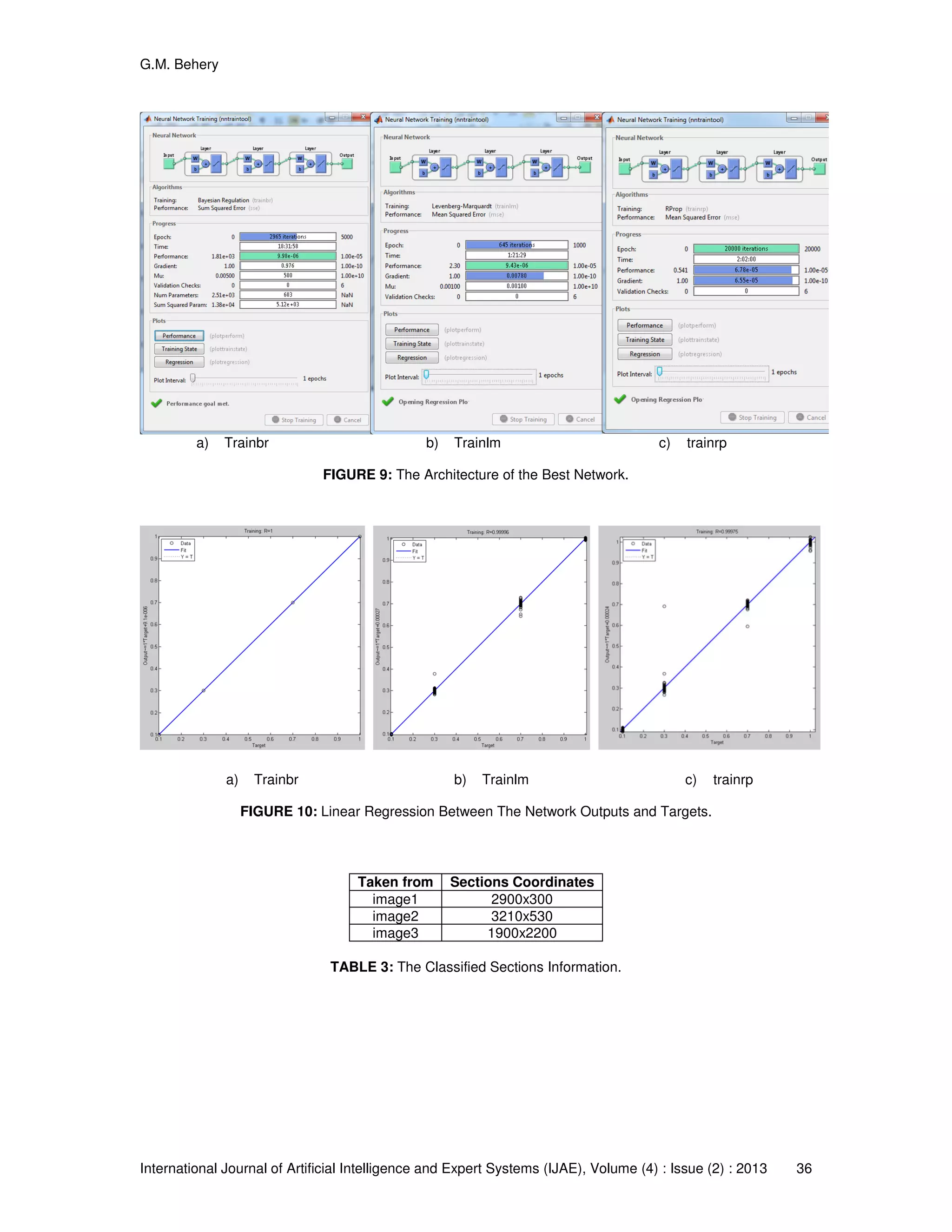
for finding the best network. The proposed systemdid many tries to find the best networksusing
low number of hidden layers and neurons. It was found that, two hidden layers with 33 and 11
neurons are enough for reaching the optimal solution.The performances of the best three training
functions (trainbr, trainlm and trainrp) on the test data were %99.82, %99.64, and %99.28
respectively. Although, the proposed system was trained on data selected only from the
image2,thissystem shows an excellent classificationofall features in the other two images.
Moreover, the proposed system can simulate the other distributions not presented in the training
set and matched them effectively.The system can store the obtained networks including the
weighted and biases values. Thus provides the system to make the test and classification
process without retraining again.
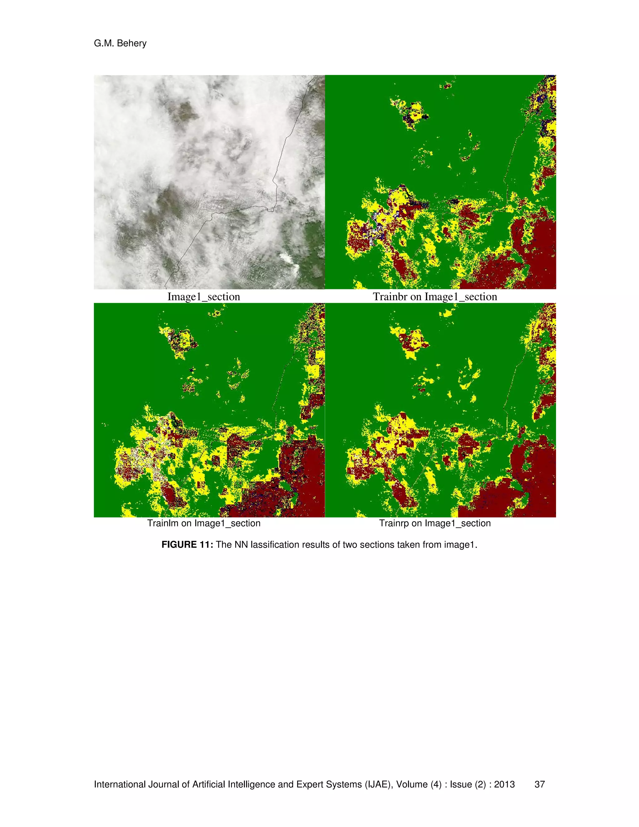
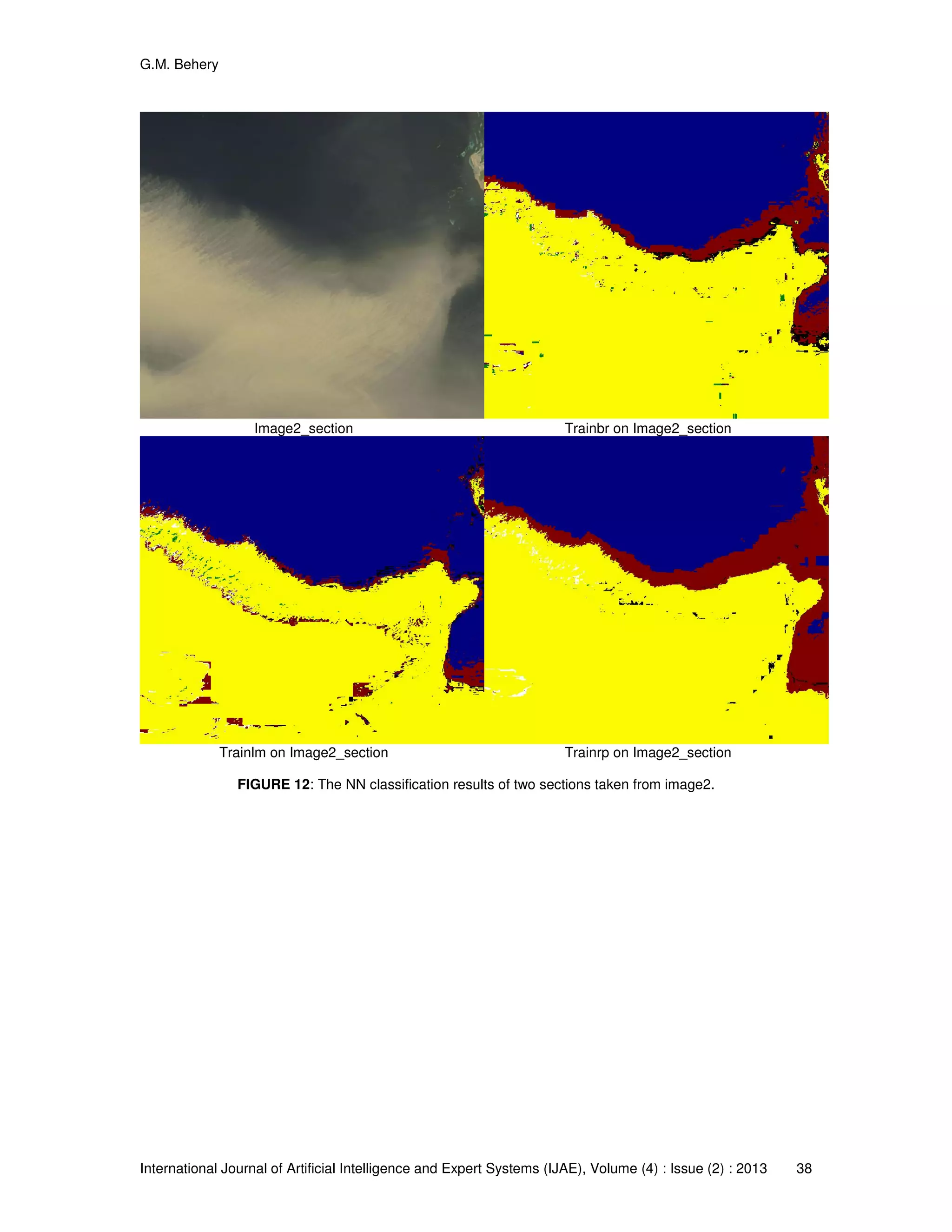
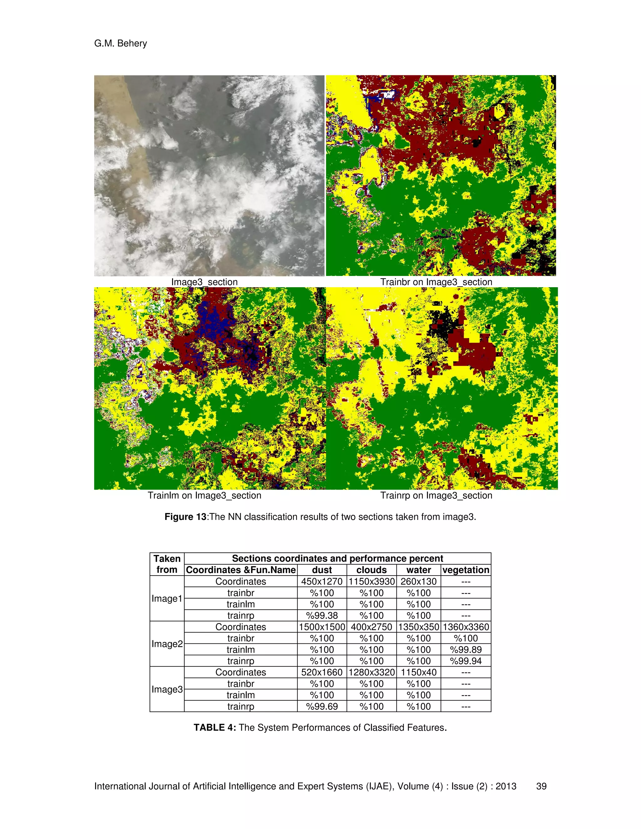
In order to calculate the classification performance of the best network on the features data, the
proposed system was applied on some small sections that were selected from contiguous areas
contained the specified features. The best networkswere applied on these sections, it was found
that the proposed system was classified the clouds and water features from the three images
correctly. It was noticed that the system was classified the dust feature correctly from the image2
that was used for collecting the training data. While,the other two images had some pixels that
were mis-classified.
6. FUTURE WORK
This system can be improved with decreasing processing time of training by using the weighting
values for previous experiment as initial weighting values for the next experiment.
7. REFERENCES
[1] L. Bai, H. Lin, H. Sun, Z.Zang, and D. Mo. "Remotely Sensed Percent Tree Cover Mapping Using
Support Vector Machine Combined with Autonomous Endmember Extraction". Physics Procedia, vol.
33, pp. 1702-1709, 2012.
[2] J. Roberts, S.Tesfamichael, M. Gebreslasie, J. Aardt and F. Ahmed. "Forest structural assessment
using remote sensing technologies: an overview of the current state of the art". Southern Hemisphere
Forestry Journal 2007, vol. 69(3), pp.183-203, 2007.

G.M. Behery
[3] M. Choi, J. M. Jacobs, M. C. Anderson, and D. D. Bosch. "Evaluation of drought indices via remotely
sensed data with hydrological variables". Journal of Hydrology, vol. 476, pp. 265-273, 2013.
[4] O.R. Abd El-Kawy, J.K. Rød, H.A. Ismail, and A.S. Suliman."Land use and land cover change
detection in the western Nile delta of Egypt using remote sensing data". Applied Geography, vol. 31(2),
pp. 483-494, 2011.
[5] P. S. Thenkabail, M. Schull, and H. Turral."Ganges and Indus river basin land use/land cover (LULC)
and irrigated area mapping using continuous streams of MODIS data". Remote Sensing of Environment,
vol. 95(3), pp. 317-341, 2005.
[6] A. Halder, A. Ghosh, and S. Ghosh. "Supervised and unsupervised landuse map generation from
remotely sensed images using ant based systems". Applied Soft Computing, vol. 11, pp. 5770-5781,
2011.
[7] Y. Kamarianakis, H. Feidas, G. Kokolatos, N. Chrysoulakis, and V. Karatzias. "Evaluating remotely
sensed rainfall estimates using nonlinear mixed models and geographically weighted regression".
Environmental Modelling& Software, vol. 23, pp. 1438-1447, 2008.
[8] G. M. Foody. "Assessing the accuracy of land cover change with imperfect ground reference data".
Remote Sensing of Environment, vol. 114(10), pp. 2271-2285, 2010.
[9] L. Huang, J. Li, D. Zhao, and J. Zhu."A fieldwork study on the diurnal changes of urban microclimate
in four types of ground cover and urban heat island of Nanjing, China". Building and Environment, vol.
43(1), pp. 7-17, 2008.
[10] J. O. Adegoke, R. Pielke, and A. M. Carleton."Observational and modeling studies of the impacts of
agriculture-related land use change on planetary boundary layer processes in the central U.S.".
Agricultural and Forest Meteorology, vol. 142(2-4), pp. 203-215, 2007.
[11] T. M. Kuplich. "Classifying regenerating forest stages in Amazoˆnia using remotely sensed images
and a neural network". Forest Ecology and Management, vol. 234, pp.1-9, 2006.
[12] Y. Ren, J. Yan, X. Wei, Y. Wang, Y. Yang, L. Hua, Y. Xiong, X. Niu, and X. Song. "Effects of rapid
urban sprawl on urban forest carbon stocks: Integrating remotely sensed, GIS and forest inventory
data". Journal of Environmental Management, vol. 113, pp.447-455, 2012.
[13] J. Franklin, L.A. Spears-Lebrun, D.H. Deutschman and K. Marsden."Impact of a high-intensity fire
on mixed evergreen and mixed conifer forests in the Peninsular Ranges of southern California, USA".
Forest Ecology and Management, vol. 235(1-3), pp. 18-29, 2006.
[14] J. N.Schwarz, B. Raymond, G.D. Williams, B. D. Pasquer, S. J.Marsland, and R.J. Gorton.
"Biophysical coupling in remotely-sensed wind stress, sea surface temperature, sea ice and chlorophyll
concentrations in the South Indian Ocean". Deep-Sea Research II, vol. 57, pp. 701-722, 2010.
[15] X.A. Padin, G. Navarro, M. Gilcoto, A.F. Rios, and F.F. Pérez. "Estimation of air–sea CO2 fluxes in
the Bay of Biscay based on empirical relationships and remotely sensed observations". Journal of
Marine Systems, vol. 75, pp. 280-289, 2009.
[16] F. Ling, X. Li, F. Xiao, S. Fang, and Y. Du. "Object-based sub-pixel mapping of buildings
incorporating the prior shape information from remotely sensed imagery". International Journal of
Applied Earth Observation and Geoinformation, vol. 18, pp.283-292, 2012.
[17] A.A. El-Harby. "Automatic classification System of Fires and smokes from the Delta area in Egypt
using Neural Networks". International Journal of Intelligent Computing and Information Science (IJICIS),
vol. 8(1), pp. 59-68, 2008.

G.M. Behery
[18] J. Zhang, L.Gruenwald, and M. Gertz."VDM-RS: A visual data mining system for exploring and
classifying remotely sensed images". Computers & Geosciences, vol. 35(9), pp. 1827-1836, 2009.
[19] K. Liu, W. Shi, and H. Zhang."A fuzzy topology-based maximum likelihood classification". ISPRS
Journal of Photogrammetry and Remote Sensing, vol. 66(1), pp. 103-114, 2011.
[20] T. KAVZOGLU and C. A. O. VIEIRA."An Analysis of Artificial Neural Network Pruning Algorithms in
Relation to Land Cover Classification Accuracy". In Proceedings of the Remote Sensing Society
Student Conference, Oxford, UK, 1998, pp. 53-58.
[21] Y. Hu, and J. Tsai."Backpropagation multi-layer perceptron for incomplete pairwise comparison
matrices in analytic hierarchy process". Applied Mathematics and Computation, vol. 180(1), pp. 53-62,
2006.
[22] X.G. Wang, Z. Tang, H. Tamura, M. Ishii and W.D. Sun."An improved backpropagation algorithm to
avoid the local minima problem".Neurocomputing, vol. 56, pp. 455-460, 2004.
[23] Z. Chen, Z. Chi, H. Fu, and D. Feng. "Multi-instance multi-label image classification: A neural
approach". Neurocomputing, vol. 99, pp. 298-306, 2013.
[24] A.A. El-Harby. "Automatic extraction of vector representation of line features: Classifying from
remotely sensed images". LAMBERT Academic Publishing AG & Co. KG (Germany), U.S.A. & U.K,
2010.
[25] M. Y. El-Bakry, A.A. El-Harby, and G.M. Behery. "Automatic Neural Network System for Vorticity
of Square Cylinders with Different Corner Radii". An International Journal of Applied Mathematics and
Informatics, vol. 26(5-6), pp. 911-923, 2008.
[26] A.A. El-Harby, G.M. Behery, and Mostafa.Y. El-Bakry, "A Self-Reorganizing Neural Network
System", WCST, August 13-15, Vienna, Austria, 2008.
[27] G.M. Behery, A.A. El-Harby, and M.Y. El-Bakry. "Reorganizing Neural Network System for Two-
Spirals and Linear-Low-Density Polyethylene Copolymer problems". Applied Computational Intelligence
and Soft Computing, vol. 2009, pp. 1-11, 2009.
[28] C. Igel and M. Hüsken."Empirical evaluation of the improved Rprop learning
algorithms".Neurocomputing, vol. 50, pp. 105-123, 2003.
[29] A.A El-Harby, "Automatic extraction of vector representations of line features from remotely sensed
images", PhD Thesis, Keele University, UK, 2001.
[30] M. Riedmiller, and H. Braun. "A direct adaptive method for faster Backpropagation learning: The
RPROP algorithm". in H. Ruspini, ed., Proc. IEEE Internet Conf. On Neural Networks (ICNN), San
Francisco, 1993, pp. 586-591.
[31] http://www.eoimages.gsfc.nasa.gov/images/imagerecords/44000/44777/redsea_tmo_2010205_lrg.jpg
[34] Q. Miao, L. Bian, X. Wang, and C. Xu. "Study on Building and Modeling of Virtual Data of Xiaosha
River Artificial Wetland". Journal of Environmental Protection, vol. 4, pp. 48-50, 2013.
[35] A. Neyamadpour, S. Taib, and W.A.T.W.Abdullah. "Using artificial neural networks to invert 2D DC
resistivity imaging data for high resistivity contrast regions: A MATLAB application". Computers &

G.M. Behery
Geosciences vol. 35, pp. 2268-2274, 2009.
[36] L. Momenzadeh, A.Zomorodian, and D. Mowla. "Experimental and theoretical investigation of
shelled corn drying in a microwave-assisted fluidized bed dryer using Artificial Neural Network". Food
and Bioproductsprocessing , vol. 8 (9) , pp. 15-21, 2 0 1 1.
[37] P.P. Tripathy,and S. Kumar. "Neural network approach for food temperature prediction during solar
drying". International Journal of Thermal Sciences vol., 48, pp. 1452-1459, 2009.
[38] S.Pandey, D.A. Hindoliyab, and R. Mod, "Artificial neural networks for predicting indoor temperature
using roof passive cooling techniques in buildings in different climatic conditions". Applied Soft
Computing vol. 12, pp. 1214-1226, 2012.
[39] M. K. D.Kiani, B. Ghobadian, T. Tavakoli, A.M. Nikbakht, and G. Najafi. "Application of artificial
neural networks for the prediction of performance and exhaust emissions in SI engine using ethanol-
gasoline blends". Energy vol. 35 pp. 65-69, 2010.
[40] A.Pandey, J. K. Srivastava, N. S. Rajput, and R. Prasad. "Crop Parameter Estimation of Lady
Finger by Using Different Neural Network Training Algorithms". Russian Agricultural Sciences, vol. 36,
No. 1, pp. 71-77, 2010.
[41] H. Parmar,and D.A. Hindoliya. "Artificial neural network based modelling of desiccant wheel".
Energy and Buildings vol.43, pp. 3505-3513, 2011.
[42] N. A. Darwish,and N. Hilal. "Sensitivity analysis and faults diagnosis using artificial neural networks
in natural gas TEG-dehydration plants". Chemical Engineering Journal vol. 137, pp. 189-197, 2008.
[43] X. Xi, Y. Cui, Z. Wang, J. Qian, J. Wang, L. Yang , and S. Zhao. "Study of dead-end microfiltration
features in sequencing batch reactor (SBR) byoptimized neural networks". Desalination vol. 272, pp.
27-35 2011.
[44] A. M. Zain, H. Haron, and S. Sharif. "Prediction of surface roughness in the end milling machining
using Artificial Neural Network". Expert Systems withApplications vol. 37, pp.1755-1768, 2010.
[45] S. Mehrotra, O.Prakash, B. N. Mishra, and B. Dwevedi. " Efficiency of neural networks for prediction
of in vitro culture conditions and inoculum properties for optimum productivity". Plant Cell Tiss Organ
Cult , vol. 95, pp. 29-35, 2008.
[46] A. J. Torija, D. P. Ruiz, and A.F. Ramos-Ridao." Use of back-propagation neural networks to predict
both level and temporal-spectral composition of sound pressure in urban sound environments". Building
and Environment vol. 52, pp. 45-56, 2012.
[47] J. A. Mumford, B. O. Turner, F. G. Ashby, and R. A. Poldrack." Deconvolving BOLD activation in
event-related designs for multivoxel patternclassification analyses".NeuroImage vol. 59, pp. 2636-2643,
2012.
[48] Z.Rongqun, Z.Daolin. "Study of land cover classification based on knowledge rules using
high-resolution remote sensing images", Expert Systems with Applications vol. 38, pp. 3647–
3652, 2011.
[49] L. Yu, A. Porwal, E. Holden, and M. C.Dentith."Towards automatic lithological classification
from remote sensing data using support vector machines", Computers & Geosciences vol. 45, pp.
229–239, 2012.

G.M. Behery
[50] K. Mori, T. Yamaguchi, J. G. Park, K. J. Mackin. "Application of neural network swarm
optimization for paddy-field classification from remote sensing data", Artif Life Robotics, vol. 16,
pp. 497–501, 2012.

An Automatic Neural Networks System for Classifying Dust, Clouds, Water, and Vegetation from Red Sea Area

More Related Content

What's hot

Viewers also liked

Similar to An Automatic Neural Networks System for Classifying Dust, Clouds, Water, and Vegetation from Red Sea Area

More from Waqas Tariq

Recently uploaded

An Automatic Neural Networks System for Classifying Dust, Clouds, Water, and Vegetation from Red Sea Area