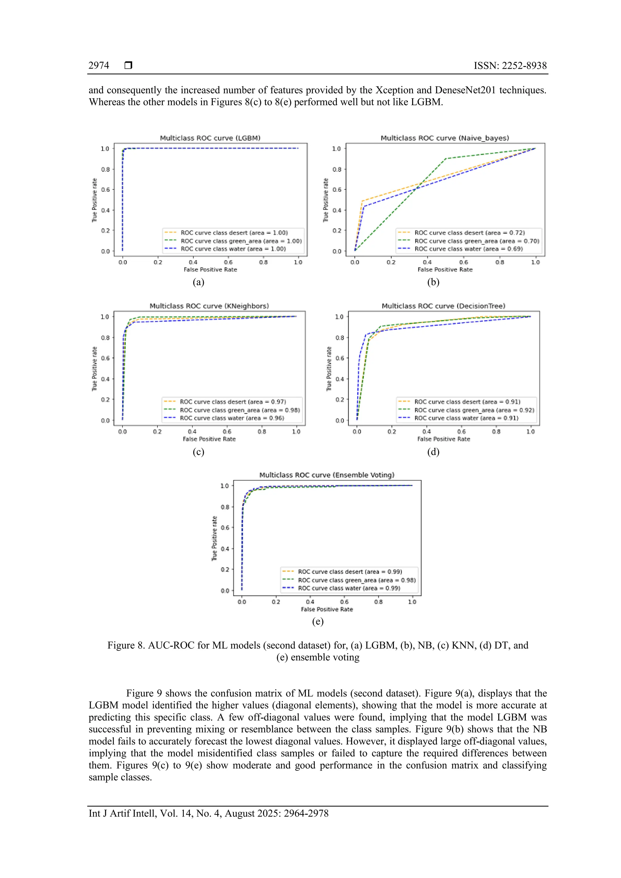
Deserts cover a significant portion of the earth and present environmental and economic difficulties owing to their harsh conditions. Satellite remote sensing images (SRSI) have evolved into an important tool for monitoring and studying these regions as technology has advanced. Machine learning (ML) is critical in evaluating these images and extracting valuable information from them, resulting in a better knowledge of hard settings and increasing efforts toward sustainable development in desert regions. As a result, in this study, four ML approaches were enhanced by hybridizing them with pre-training methods to achieve multi model learning. Two pre-training approaches (Xception and DeneseNet201) were used to extract features, which were concatenated and fed into ML algorithms: light gradient boosting model (LGBM), decision tree (DT), k-nearest neighbors (KNN), and naïve Bayes (NB). In addition, an ensemble voting was used to improve the outcomes of ML algorithms (DT, NB, and KNN) and overcome their flaws. The models were tested on two datasets and hybrid LGBM outperformed other traditional ML methods by 99% in accuracy, precision, recall, and F1 score, and by 100% in area under the curve (AUC)-receiver operating characteristic (ROC).

1. IAES International Journal of Artificial Intelligence (IJ-AI)
Vol. 14, No. 4, August 2025, pp. 2964~2978
ISSN: 2252-8938, DOI: 10.11591/ijai.v14.i4.pp2964-2978  2964
Journal homepage: http://ijai.iaescore.com
Enhancing traditional machine learning methods using
concatenation two transfer learning for classification desert
regions
Rafal Nazar Younes Al-Tahan1
, Ruba Talal Ibrahim2
1
Department of Computer Science, The General Directorate of Education in Nineveh Governorate, Mosul, Iraq
2
Department of Computer Science, College of Computer Science and Mathematics, University of Mosul, Mosul, Iraq
Article Info ABSTRACT
Article history:
Received Sep 11, 2024
Revised Apr 15, 2025
Accepted Jun 8, 2025
Deserts cover a significant portion of the earth and present environmental
and economic difficulties owing to their harsh conditions. Satellite remote
sensing images (SRSI) have evolved into an important tool for monitoring
and studying these regions as technology has advanced. Machine learning
(ML) is critical in evaluating these images and extracting valuable
information from them, resulting in a better knowledge of hard settings and
increasing efforts toward sustainable development in desert regions. As a
result, in this study, four ML approaches were enhanced by hybridizing them
with pre-training methods to achieve multi model learning. Two pre-training
approaches (Xception and DeneseNet201) were used to extract features,
which were concatenated and fed into ML algorithms: light gradient
boosting model (LGBM), decision tree (DT), k-nearest neighbors (KNN),
and naïve Bayes (NB). In addition, an ensemble voting was used to improve
the outcomes of ML algorithms (DT, NB, and KNN) and overcome their
flaws. The models were tested on two datasets and hybrid LGBM
outperformed other traditional ML methods by 99% in accuracy, precision,
recall, and F1 score, and by 100% in area under the curve (AUC)-receiver
operating characteristic (ROC).
Keywords:
Decision tree
DenseNet201
K-nearest neighbor
Light gradient boosting model
Machine learning
Satellite remote sensing images
Xception
This is an open access article under the CC BY-SA license.
Corresponding Author:
Ruba Talal Ibrahim
Department of Computer Science, College of Computer Science and Mathematics, University of Mosul
Al-Hadbaa Road-Mosul, Iraq
Email: rubatalal@uomosul.edu.iq
1. INTRODUCTION
Our planet Earth is made up of 29% land (continents and islands), with the remaining 71%
controlled by water [1]. The land is then separated into two categories: lands suited for habitation and
agriculture (green meadows) and barren desert grounds that are unsuitable for both [2]. Desertification is a
natural phenomenon that causes land deterioration owing to wind and drifting sand. It is one of the
environmental disasters that must be prevented or mitigated by knowing its dynamic growth and extent, as
well as examining climatic and geographical topology such as temperature, plant cover, rainfall rate,
latitude, and longitude [3]. In recent decades, remote sensing satellites have been able to record the Earth's
topology, resulting in remote sensing images with high resolution and advanced processing, as well as low
prices and rapid acquisition [4]. Researchers have been able to use these images in many important
research fields such as environmental monitoring [5], navigation and mapping [6], Google Earth and
OpenStreetMap [7]. Manual classification of natural regions using geographic information systems or
remote sensing is exceedingly challenging owing to a lack of understanding of their surface, geography,

2. Int J Artif Intell ISSN: 2252-8938 
Enhancing traditional machine learning methods using concatenation … (Rafal Nazar Younes Al-Tahan)
2965
and changing illumination, all of which have resulted in a constant change in the features of these regions,
especially desert regions. Therefore, an electronic classification has become necessary because it does not
require time, effort, and field experts, unlike manual classification, which also requires high cost of
localization and the willingness of data analysis to undertake less research. In recent years, machine
learning (ML) techniques have emerged to classify natural regions using remote sensing images and have
achieved good results [8]. Many researchers have used pre-trained ML methods to classify desert, green,
and water regions and have achieved excellent results, but some of them have faced problems such as
overfitting, which has affected the accuracy [9]. To reduce the spread of desert regions and the
phenomenon of desertification that has increased recently and to encourage sustainable agriculture this
study investigated to classify natural regions (desert, green, and water) and detects desert regions in
particular, in addition to improving the quality of traditional ML techniques due to their saturation when
classifying a large amount of data, as well as to avoid overfitting, which usually occurs in pre-trained
learning that acquires weights and biases that represent the characteristics of the data set. So, traditional
and modern ML methods were hybridized with two pre-trained learning methods, Xception and
DenseNet201, to extract features and achieve high-quality and multi-model learning while previous studies
have not addressed this. These features were then passed to more than one ML technique to be classified.
Additionally, an ensemble method was used between more ML methods to improve accuracy. The paper's
contributions can be summarized in the following points:
‒ Applying two datasets, first satellite remote sensing images (SRSI) was taken from Kaggle website
and, the second dataset was collected from many websites like: Kaggle, NASA, and Nimbo. Also,
only three classes were taken from the two datasets, which are (desert, green areas, and water).
‒ Performing many preprocessing on the two datasets, such as (resizing images, transformation, canny
detection, bounding box images, cropping images, and normalization).
‒ Applying two transfer learning techniques (Xception and DenseNet201) to extract features and
accomplish multi-model learning.
‒ After concatenating the transfer learning outcomes, the multi-features will be fed into traditional and
modern ML algorithms such as (light gradient boosting model (LGBM), decision tree (DT), k-nearest
neighbors (KNN), and naïve Bayes (NB)). additionally, the work used an ensemble voting method
amongst three traditional ML algorithms to improve accuracy and performance.
The remainder of the study is structured as follows: section 2 will address related works.
Sections 3 and 4 will offer transfer learning and ML methods. Section 5 will describe research
methodology. Section 6 will present evaluation methods. Finally, section 7 will offer the results and
discussions, followed by section 8, which is the conclusion.
2. RELATED WORK
Many researchers have focused their efforts on using ML to classify natural regions or SRSI
images. In 2017 Pritt and Chern [10] proposed deep learning system using convolutional neural networks
(CNN) which classified objects in high-resolution satellite imagery from the IARPA functional map of the
world (fMoW) dataset into 63 classes with 83% accuracy. It integrated image features and metadata,
achieving second place in the fMoW TopCoder competition and the system achieved 95% or higher
accuracy in 15 classes and placed second in the fMoW TopCoder challenge with a score of 765,663.
In 2018 Buscombe and Ritchie [11] introduced a method for efficiently training deep CNNs
(DCNNs) using conditional random fields (CRFs) with minimal manual supervision to classify natural
landscapes. It demonstrated the approach's effectiveness in landscape-scale image classification and
highlights its potential for accurate pixel-level classification using transfer learning, and it presented a
workflow for efficiently creating labeled imagery and retraining DCNNs for semantic classification. The
workflow, using MobileNetV2, achieved high classification accuracies (91 to 98%) across various
datasets.
In 2020, Lee et al. [12] used deep learning to classify human-induced deforestation, it found that
U-Net outperformed SegNet in accuracy (74.8% vs. 63.3%), particularly in distinguishing forest from
non-forest areas. By constructing precise training datasets, 13 classes were formed to distinguish forest
and non-forest areas. The study highlights the potential of deep-learning models in analyzing
deforestation, while acknowledging the need for more advanced algorithms and larger datasets for
improved accuracy and broader application. Also, in 2020, Haq et al. [13] demonstrated the effectiveness
of deep learning-based supervised image classification using unmanned aerial vehicle (UAV)-collected
data for forest area classification. It highlighted the significant role of UAVs and deep learning in
managing and planning forest areas threatened by deforestation. The results showed that an accuracy was
93.28% and a Kappa coefficient was 0.8988. In 2020, Rahman et al. [14] evaluated the performance of
ML algorithms (random forest, support vector machine (SVM), and stacked algorithms) on classifying

3.  ISSN: 2252-8938
Int J Artif Intell, Vol. 14, No. 4, August 2025: 2964-2978
2966
land use and land cover changes using landsat-8, sentinel-2, and planet images in rural and urban areas.
The sentinel-2 image with SVM performed best, achieving high accuracy, aiding in monitoring fragmented
landscapes in Bangladesh and beyond and found that its sentinel-2 imagery outperforms landsat-8 and
planet in accuracy, with the SVM achieving the highest results when used with sentinel-2 data. In both
Bhola (rural) and Dhaka (urban), SVM provided the highest overall accuracy (0.969 and 0.983) and Kappa
values (0.948 and 0.968). In 2022, Gevaert and Belgiu [15] proposed landscape metrics to assess the
similarity between training and testing images for building identification with fully convolutional
networks (FCNs). The model trained on Dares Salaam images showed the highest generalization, while the
Zanzibar-trained model had the lowest. The classification accuracies are lower than those in the open cities
AI challenge due to limited training data for evaluating generalizability. This study focuses on identifying
image similarity metrics that predict model performance rather than achieving maximum accuracy. In
2023, Chaudhari et al. [16] explored drought prediction using satellite images and deep learning models.
They compared EfficientNet with other CNN variants like AlexNet and visual geometry group network
(VGGNet). It found that EfficientNet outperforms these models which achieve higher accuracy in binary
drought classification, and found that variants of CNN are commonly used in image processing. This study
evaluated their effectiveness for drought classification using satellite images from Kolar, Karnataka and
EfficientNet outperforms traditional CNN models like CNN, AlexNet, and VGGNet, achieving higher
accuracies of 0.91 to 0.94. Despite CNN's superior performance with an accuracy of 0.97, all models need
extended training periods.
3. TRANSFER LEARNING
3.1. Xception transfer learning
The Xception model is a pre-training model on the ImageNet dataset. The model was recently
designed as an extension of the Inceptionv3 model. It was invented by Chollet [17]. It is more robust and has
less overfitting difficulties than current popular pre-training models like VGG16 [18].
Xception model is based on the principle of depth-wise separable convolution instead of classic
convolution. The depth-wise separable convolution passes through two stages that are applied in reverse
manner. First stage called depth wise convolution which does not apply a convolutional filter to all channels
at the same time, but rather applies it to each input channel for reducing computations and memory space
used. Second stage called Pointwise convolution which integrate the first stage depth wise convolution output
over all channels by using a 1×1 convolution [19].
According to Figure 1, the Xception architecture consists of three primary parts. The first called
entry flow, which is where the data is first processed. The data is subsequently sent via the middle flow,
which is repeated eight times, and lastly through the exit flow.
Figure 1. Xception architecture

4. Int J Artif Intell ISSN: 2252-8938 
Enhancing traditional machine learning methods using concatenation … (Rafal Nazar Younes Al-Tahan)
2967
Figure 1 showed that three blocks consist of convolution layers with a number of rectified linear unit
(ReLU) and max-pooling layers between them. The entry flow block consists of eight convolution layers,
while the middle flow block consists of 24, and finally the exit flow block consists of four convolution layers.
After that, the global average pooling layer followed the convolution layers to convert to the fully connected
layer which reduced the number of parameters.
3.2. DenseNet201 transfer learning
It is a transfer learning model trained on the ImageNet dataset and built on the CNN principles.
It was proposed by Huang et al. [20] and was utilized in various major fields of artificial intelligence,
including object detection and classification, due to its capacity to reuse features and reduce the problem of
vanishing gradients, as well as its usage of a limited number of features. DenseNet201 relies on a simple
strategy, which is to connect all layers in a feed-forward way so that each layer is fed from all previous layers
and also passes its feature maps to subsequent layers [21]. DenseNet201's key components are dense blocks
and transition layers (see Figure 2).
Figure 2. DenseNet201 architecture
The fundamental feature of the model network is dense blocks, which are made up of several
bottleneck layers. Information from each layer is connected via the dense connection mode inside the dense
block, guaranteeing that the output size remains consistent throughout. DenseNet controls the amount of
channels using bottleneck layers, transition layers, and a growth rate [22].
4. MACHINE LEARNING
4.1. Naïve Bayes algorithm
It is named NB because the computations of the probability for each class are reduced to make its
computation tractable. It is famous in multiclassification domain. NB classifiers rely on Bayesian
algorithms [23]. These are based on Bayes' theorem, an equation that describes the relationship between
the conditional probabilities of statistical data. In Bayesian classification, we want to know the probability
of a label given some observable characteristics [24]. In other words, it explains the likelihood of an event
occurring given on past knowledge of the occurrence of another event. To make the forecast, compute
P(A|B), which is the likelihood of A occurring if B is true. Furthermore, P(B|A) represents the likelihood
of B occurring if A is true. P(B) and P(A) are the probability of seeing one without the other, as illustrated
in (1) [25].
𝑃(𝐴|𝐵) =
𝑃(𝐵|𝐴) 𝑃(𝐴)
𝑃(𝐵)
(1)

5.  ISSN: 2252-8938
Int J Artif Intell, Vol. 14, No. 4, August 2025: 2964-2978
2968
4.2. Decision tree algorithm
In public life, while considering a specific topic and making a decision, one must carefully
consider all of the advantages and downsides of the option or the alternatives available. Similarly, in ML,
DT do the same function with more precision, taking into account all relevant variables to make the
optimal decision [26]. DT are a powerful tool utilized in a variety of domains, including classification,
image processing, and pattern recognition [27]. It may be used as statistical processes to discover data,
extract text, identify missing data in a class, enhance search engines, and has a variety of medicinal uses
[28]. It consists of root nodes (top nodes), branches (links), and leaf nodes. In a DT, testing takes place on
the interior nodes, and the output is performed on the leaf nodes. Each node represents a feature, each
branch is accountable for the decision, and each leaf displays the result. The way DT work is that, each
internal node divides the dataset into subsets depending on a feature criterion. The objective is to make the
subsets as pure as possible, which means they should only include data points from the same
categorization class. The most criterion functions in DT used are: Gini index and entropy measures. When
an element is randomly classified according to the distribution of labeled in the set, the Gini index
measures the probability of incorrectly classifying that element.
4.3. K-nearest neighbors algorithm
KNN is a widely used supervised ML algorithm, particularly effective for classification and
regression tasks. The fundamental principle behind KNN is that similar instances are likely to exist close to
each other within the feature space, allowing for the categorization of new samples based on their proximity
to already classified data points (neighbors) [29]. The most common distance metrics used in KNN include
Euclidean distance, Manhattan distance, Minkowski distance, cosine similarity, and correlation [29].
Among these, Euclidean distance is particularly well-known and is mathematically defined as the straight-
line distance between two points in a multidimensional space.
4.4. Light gradient boosting machine
Gradient boosting machines (GBMs) are a type of ensemble learning method that construct an
additive model from simple DT. These trees, which are not highly optimized individually, are then combined
by optimizing a loss function, leading to stronger predictive performance [30]. LightGBM offers faster
training speeds and greater efficiency than many other algorithms. This is primarily due to its histogram-
based approach, which buckets continuous feature values into discrete bins, thereby accelerating the training
process. LightGBM uses a leaf-wise algorithm to grow trees vertically, selecting the leaf that most reduces
the loss for splitting. To optimize training, LightGBM employs a technique called gradient-based one-side
sampling (GOSS), which focuses on data instances with larger gradients, assuming that instances with
smaller gradients are already well-trained and can be ignored.
5. RESEARCH METHODOLOGY
The proposed methodology consisted of many steps: pre-processing and feature, followed by
classification process using both traditional and state of art ML techniques like: DT, NB, KNN, LGBM, and
ensemble voting. Figure 3 shows the workflow of the proposed methodology which applied on Windows 10
and 4-core CPU with a processing speed of 2.00 GHz. Memory capacity of 16.0 GB.
5.1. Description of dataset
The proposed models were tested on two SRSI datasets for generalization purposes. The first dataset
was taken from the Kaggle website and consists of (4,131) images classified into only three classes
(desert, green_area, and water). The second dataset is similar to the first dataset, but it includes extra data
from several sources such as the Kaggle website [31], NASA [32] and Nimbo [33] to balance three classes.
The total number of images was (6,900) images over three classes. The data was split into 80% training and
20% testing.
5.2. Image pre-processing
Preprocessing is an essential step for finding relevant features in SRSI and ensuring that the data is
ready for certain kind of analysis. Figure 4 depicts many procedures that were performed to digital images:
‒ Resize images: It is a vital step in ensuring that all images are uniform and of equal size.
Furthermore, lowering the number of pixels in images will minimize the number of processors and
memory required. In this work, the resize function in Python was used to uniformly scale the images
to 150 width * 150 heights.

6. Int J Artif Intell ISSN: 2252-8938 
Enhancing traditional machine learning methods using concatenation … (Rafal Nazar Younes Al-Tahan)
2969
‒ Image transform: OpenCV is a popular Python library for digital image processing. This library
includes (cvtColor function), which converts images from BGR color space to RGB for clarity and
simple display using the matplotlib library.
‒ Canny detection: The critical edges of the SRSI were highlighted and precisely analyzed using the
canny edge approach [34].
‒ Bounding box: It is an essential annotation approach for digital images. An abstract rectangle serves as
both an item discovery tool and a reference point for images.
‒ Cropping image: The technique of eliminating unnecessary white regions and edges from SRSI in order
to identify the edges with the most relevant elements.
‒ Normalization: It is a common image processing technique that changes the intensity range of pixels to
between 0 and 1. It is a common function to convert an input image into a range of pixel values that are
more pleasant to the human eye.
Figure 3. Workflow of proposed methodology
Figure 4. Pre-processing image

7.  ISSN: 2252-8938
Int J Artif Intell, Vol. 14, No. 4, August 2025: 2964-2978
2970
5.3. Feature extraction
Pre-trained models (Xception and DeneseNet201) were used to extract features from SRSI datasets
by passing them through numerous convolutional layers of two pre-trained models, resulting in 2D matrices
with frozen weights and removing the output layer. The characteristics of Xception transfer learning like
depth wise convolution and pointwise convolution were applied to decrease computing processes in feature
extraction. Also, DeneseNet201 connects all layers such that each layer receives input from all previous
layers while also passing on feature maps to subsequent layers. Therefore, it reduces the problem of
vanishing gradients. The concatenation process will combine the outputs of the two models in order to train
these matrices for classification using traditional and state of art ML approaches. So, concatenation process
achieved multi model learning and high-quality representation. Figure 5 shows features extracted by two
transfer learning.
Figure 5. Feature extraction after concatenate two transfer learning
5.4. Classification process
In this work, traditional and state of art ML methods (DT, NB, KNN and LGBM) were used to
classify SRSI dataset and achieve best results. Furthermore, an ensemble voting technique was applied
among three traditional ML (DT, NB, KNN) to increase the performance of model. These four ML methods
are more sensitive to relevant data, can scale with large data, is non-parametric, meaning it can adapt to the
data and does not assume a fixed model form, can interpret and extract the importance of a feature, and can
handle both categorical and numerical data. On the other hand, the hyperparameters of methods were
optimized by using grid search algorithm because it includes cross-validation, which divides the data into
k-folds for training and others for evaluation, and then repeats the process to ensure that each part of the data
is used at least once in training and evaluation. In this study, value of k-folds was 10. Table 1 displays the
important hyperparameter values.
Tuning hyperparameters are a way to avoid problems related to overfitting and underfitting. When
hyperparameter values are low, the model is unable to distinguish between the data during the training and
testing stages, resulting in underfitting. Increasing hyperparameter values leads to an overfitting and
complicated model. So, in this work a grid search method is employed to provide balanced results with fine-
tuning essential hyperparameters.

8. Int J Artif Intell ISSN: 2252-8938 
Enhancing traditional machine learning methods using concatenation … (Rafal Nazar Younes Al-Tahan)
2971
Table 1. Hyperparameters optimization
Models Hyperparameters
LGBM num_leaves=30, n_estimators=100, max_depth=7
DT Max_leaf_nodes=20, max_depth=10
NV Var_smoothing=le-9
KNN Nn_neighbors=5, leaf_size=30
Ensemble voting Voting=’soft’, n_jobs=-1
6. PERFORMANCE EVALUATION
After developing the models, their performance was evaluated using a variety of measures,
including accuracy, recall, precision, f1-score and receiver operating characteristic (ROC)-area under the
curve (AUC). Accuracy measures classification task performance by counting the number of correctly
evaluated instances across all data samples. Recall is a useful quantity measure for detecting model errors.
While precision is a quality metric that refers to the percentage of correctly identified positive instances.
The f1-score is a metric intended to strike a compromise between precision and recall. Finally,
AUC-ROC is a classification measure that determines how well a classifier distinguishes between classes at
various thresholds. It demonstrates the trade-off between specificity and sensitivity in testing that yield
numerical findings instead of a binary positive or negative conclusion. The AUC-ROC (decision thresholds)
gives the best cut-off for both sensitivity and specificity. The ROC curve for each class is displayed both the
true positive rate and false positive rate. When the AUC value for each class is 1.0, it implies perfect
discrimination, whereas 0.5 shows no discrimination i.e (random guessing). These metrics are expressed as
follows in (2) to (5) [35]:
𝑃𝑟𝑒𝑐𝑖𝑠𝑖𝑜𝑛 =
𝑇𝑃
𝑇𝑃+𝐹𝑃
(2)
𝑅𝑒𝑐𝑎𝑙𝑙 =
𝑇𝑃
𝑇𝑃+𝐹𝑃
(3)
𝐹1 − 𝑠𝑐𝑜𝑟𝑒 =
2∗𝑃𝑟𝑒𝑐𝑖𝑠𝑖𝑜𝑛∗𝑅𝑒𝑐𝑎𝑙𝑙
𝑃𝑟𝑒𝑐𝑖𝑠𝑖𝑜𝑛+𝑅𝑒𝑐𝑎𝑙𝑙
(4)
𝐴𝑐𝑐𝑢𝑟𝑎𝑐𝑦 =
𝑇𝑁 + 𝑇𝑃
𝑇𝑁 + 𝑇𝑃 + 𝐹𝑁 + 𝐹𝑃
(5)
7. RESULTS AND DISCUSSION
7.1. First dataset (satellite images)
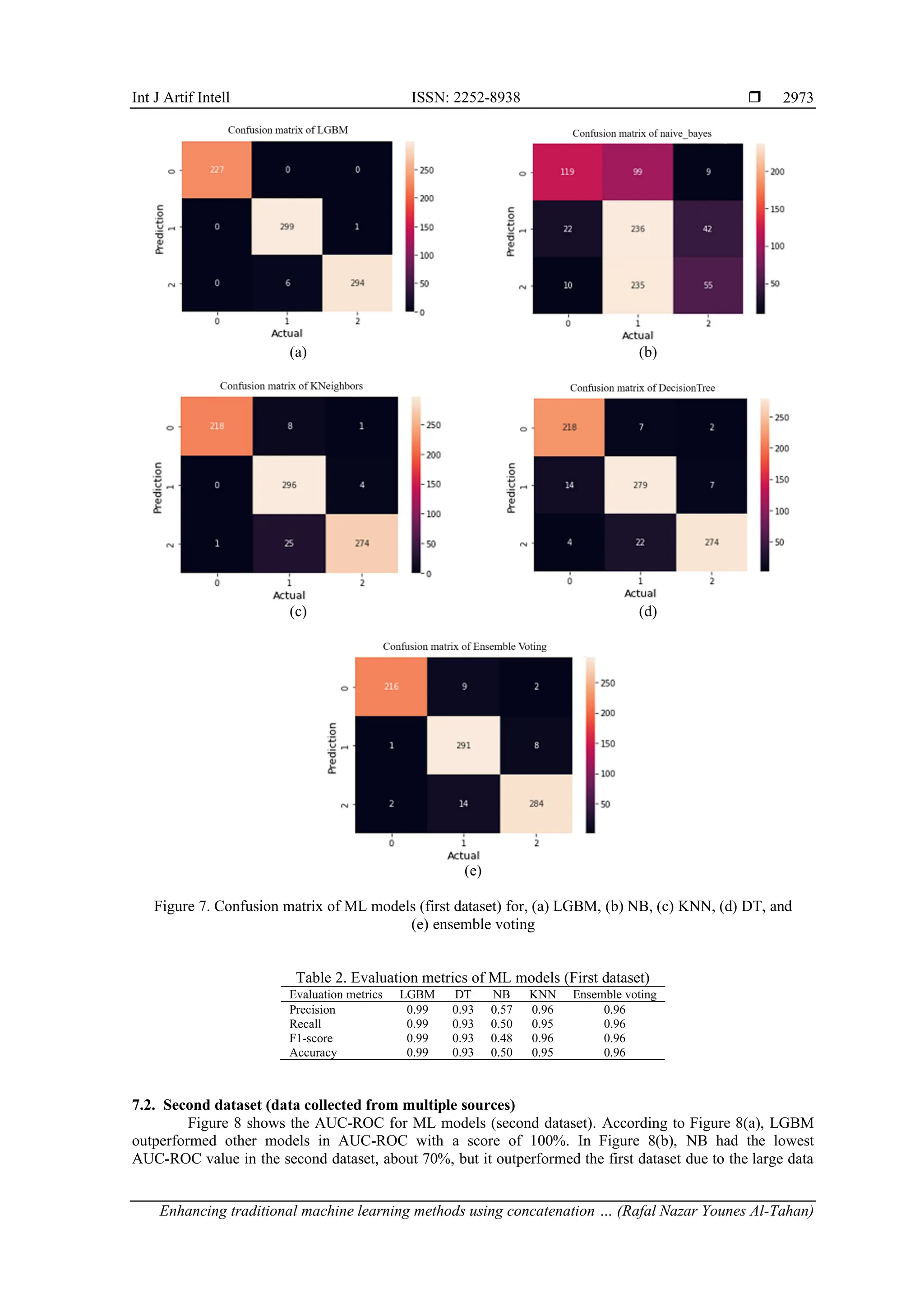
Figure 6 shows the AUC-ROC of ML models (first dataset). It was noted in Figure 6(a), that
ROC-AUC metric of the LGBM algorithm has achieved the highest percentage, which is 100% due to
LGBM decreases the cost of loss by splitting the tree into leaves rather than at the depth level employed in
prior boosting methods. Moreover, it follows parallel learning using large data to speed up the data training
process. Unlike the NB algorithm in Figure 6(b), which achieved the lowest percentage 62% among the
mentioned methods because it relies on the assumption that the features are classifying data sets with
complex hierarchical structures. As for Figures 6(c) to 6(e), they achieved best independent, and thus the
model’s predictions may be inaccurate, in addition to its being unsuitable for results in the AUC-ROC and
classify sample classes.
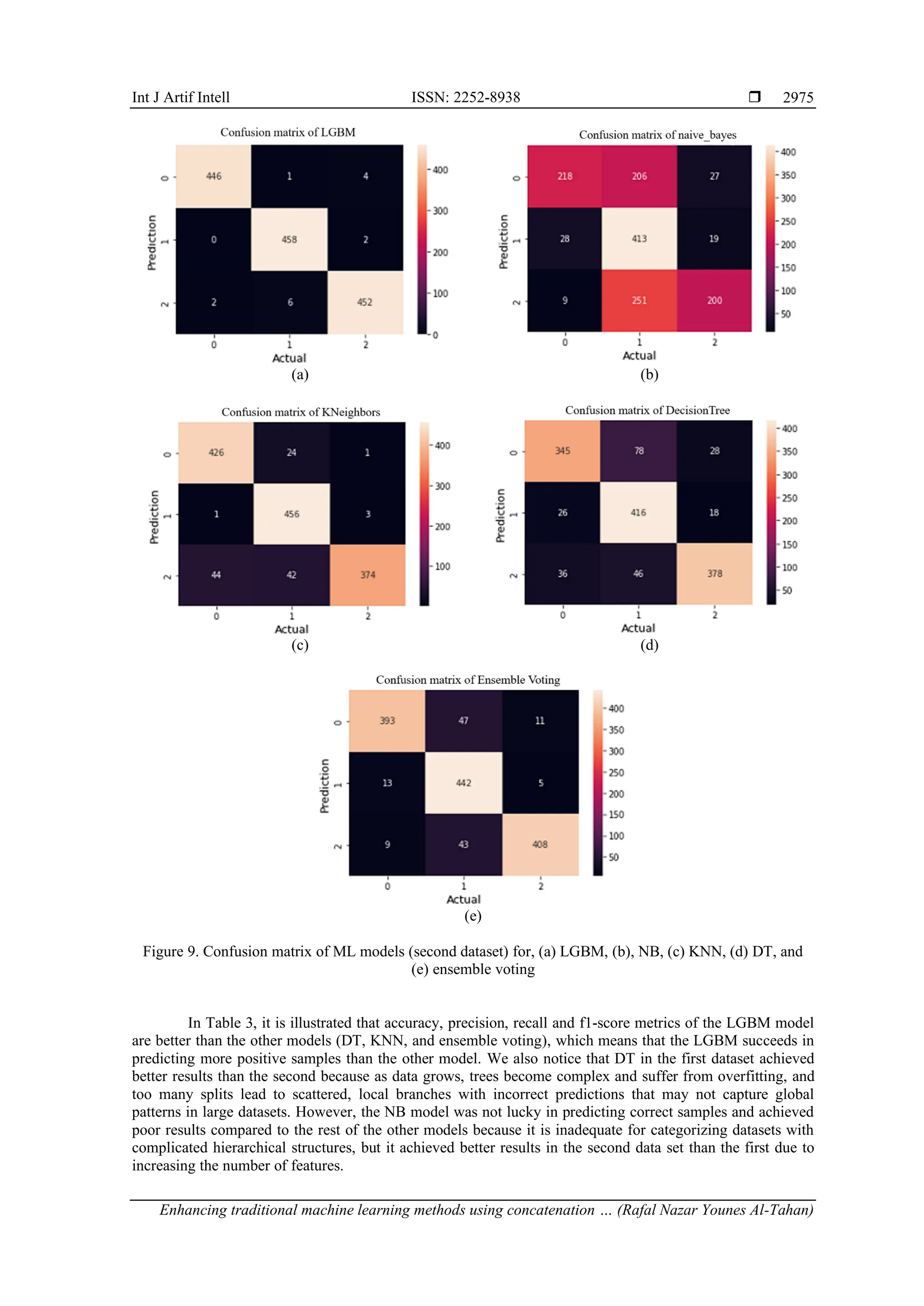
Figures 7 display the confusion matrix of SRSI classification to show more about the results and
how they change across three classes in five models. The confusion matrix shows how difficult it is for the
five models to choose between three different classes (desert, green_area, and water). It is a numerical table
that illustrated where there is confusion on a classifier. It is designed to link predictions to the original classes
to which the data belongs. It is used in supervised learning for calculating a variety of metrics in addition to
accuracy. A confusion matrix created for the same test set of a dataset but using various classifiers may also
assist analyze their relative strengths and weaknesses and draw recommendations about how to combine
them for best performance.
Also, in Figure 7(a), It was noticed that diagonal elements represent the correct predictions, so the
LGBM model classified the higher values, indicating that the model is better at predicting this specific class.
While a few off-diagonal values were observed, showing that the model LGBM succeeded in not mixing
between the class samples. In Figure 7(b), the NB model classified the lowest diagonal values, indicating that
the model is poor at predicting these specific classes. However, it showed high off-diagonal values, implying
that the model confused class samples or failed to capture the necessary distinctions between these classes.
As for Figures 7(c) to 7(e), they achieved moderate and good results and classify sample classes.

9.  ISSN: 2252-8938
Int J Artif Intell, Vol. 14, No. 4, August 2025: 2964-2978
2972
In Table 2, it was noticed that accuracy, precision, recall and f1-score metrics of the LGBM model
are better than the other models, which means that the LGBM succeeds in predicting more positive samples
(SRSI) than the other model. However, the NB model was not lucky in predicting correct samples and
achieved poor results compared to the rest of the other models because it is inadequate for categorizing
datasets with complicated hierarchical structures. As a consequence, the outcomes of traditional models
(DT, KNN, and NB) have been improved by employing ensemble voting, which combines the strengths of
each model while reducing the influence of faults in other models. In other words, it relies on merging the
findings of several models to obtain high performance and accuracy.
(a) (b)
(c) (d)
(e)
Figure 6. AUC-ROC of ML models (first dataset) for, (a) LGBM, (b) NB, (c) KNN, (d) DT, and
(e) ensemble voting

10. Int J Artif Intell ISSN: 2252-8938 
Enhancing traditional machine learning methods using concatenation … (Rafal Nazar Younes Al-Tahan)
2973
(a) (b)
(c) (d)
(e)
Figure 7. Confusion matrix of ML models (first dataset) for, (a) LGBM, (b) NB, (c) KNN, (d) DT, and
(e) ensemble voting
Table 2. Evaluation metrics of ML models (First dataset)
Evaluation metrics LGBM DT NB KNN Ensemble voting
Precision 0.99 0.93 0.57 0.96 0.96
Recall 0.99 0.93 0.50 0.95 0.96
F1-score 0.99 0.93 0.48 0.96 0.96
Accuracy 0.99 0.93 0.50 0.95 0.96
7.2. Second dataset (data collected from multiple sources)
Figure 8 shows the AUC-ROC for ML models (second dataset). According to Figure 8(a), LGBM
outperformed other models in AUC-ROC with a score of 100%. In Figure 8(b), NB had the lowest
AUC-ROC value in the second dataset, about 70%, but it outperformed the first dataset due to the large data

11.  ISSN: 2252-8938
Int J Artif Intell, Vol. 14, No. 4, August 2025: 2964-2978
2974
and consequently the increased number of features provided by the Xception and DeneseNet201 techniques.
Whereas the other models in Figures 8(c) to 8(e) performed well but not like LGBM.
(a) (b)
(c) (d)
(e)
Figure 8. AUC-ROC for ML models (second dataset) for, (a) LGBM, (b), NB, (c) KNN, (d) DT, and
(e) ensemble voting
Figure 9 shows the confusion matrix of ML models (second dataset). Figure 9(a), displays that the
LGBM model identified the higher values (diagonal elements), showing that the model is more accurate at
predicting this specific class. A few off-diagonal values were found, implying that the model LGBM was
successful in preventing mixing or resemblance between the class samples. Figure 9(b) shows that the NB
model fails to accurately forecast the lowest diagonal values. However, it displayed large off-diagonal values,
implying that the model misidentified class samples or failed to capture the required differences between
them. Figures 9(c) to 9(e) show moderate and good performance in the confusion matrix and classifying
sample classes.

12. Int J Artif Intell ISSN: 2252-8938 
Enhancing traditional machine learning methods using concatenation … (Rafal Nazar Younes Al-Tahan)
2975
(a) (b)
(c) (d)
(e)
Figure 9. Confusion matrix of ML models (second dataset) for, (a) LGBM, (b), NB, (c) KNN, (d) DT, and
(e) ensemble voting
In Table 3, it is illustrated that accuracy, precision, recall and f1-score metrics of the LGBM model
are better than the other models (DT, KNN, and ensemble voting), which means that the LGBM succeeds in
predicting more positive samples than the other model. We also notice that DT in the first dataset achieved
better results than the second because as data grows, trees become complex and suffer from overfitting, and
too many splits lead to scattered, local branches with incorrect predictions that may not capture global
patterns in large datasets. However, the NB model was not lucky in predicting correct samples and achieved
poor results compared to the rest of the other models because it is inadequate for categorizing datasets with
complicated hierarchical structures, but it achieved better results in the second data set than the first due to
increasing the number of features.

13.  ISSN: 2252-8938
Int J Artif Intell, Vol. 14, No. 4, August 2025: 2964-2978
2976
Table 3. Evaluation metrics of ML models (Second dataset)
Evaluation Metrics LGBM DT NB KNN Ensemble Voting
Precision 0.99 0.84 0.71 0.92 0.91
Recall 0.99 0.83 0.61 0.92 0.91
F1-score 0.99 0.83 0.60 0.92 0.91
Accuracy 0.99 0.83 0.60 0.92 0.91
Finally, this study examined a comprehensive relationship between ML method with transfer
learning, and LGBM method tended to have higher proportion of AUC-ROC, accuracy, confusion matrix and
other performance metrics than other (DT, NB, and KNN) models in two datasets. Also, the results of the
work were compared with a previous study [10] which used the first dataset (SRSI). Table 4 showed the
hybrid model proposed in this paper outperformed the previous study.
Table 4. Comparison with previous work
Paper Total accuracy F1 score
Pritt and Chern [10] 0.83 0.797
Proposed hybrid transfer learning+LGBM 0.99 0.99
8. CONCLUSION
Detecting desert regions is critical; decreasing them and promoting sustainable agriculture is even
more vital. Therefore, in this study, a number of ML methods were improved by hybridizing them with
pretraining methods to achieve a high-level and multi-feature model at the same time. Two transfer learning
(Xception and DeneseNet201) were used, and the extracted features were concatenated and then entered into
ML methods (LGBM, DT, KNN, and NB). Also, a tuning of important hyperparameters for ML methods was
done using grid search algorithm. In addition, an ensemble voting was applied to enhance the results of ML
algorithms (DT, NB, and KNN). The models were evaluated on two datasets, the first SRSI taken from the
Kaggle website and the second collected from several different websites. In two datasets, recent observations
indicate that hybrid LGBM with transfer learning outperformed traditional and ensemble voting methods by
99% in accuracy, precision, recall, and f1-score, and by 100% in AUC-ROC. Future studies may investigate
drought, rainfall, humidity, and temperature factors can be used as a dataset to predict natural areas.
ACKNOWLEDGMENTS
Many thanks to the Department of Computer Science, College of Computer Science and
Mathematics, University of Mosul for their support in completing the research requirements.
FUNDING INFORMATION
This research is not supported by any funding agency.
AUTHOR CONTRIBUTIONS STATEMENT
This journal uses the Contributor Roles Taxonomy (CRediT) to recognize individual author
contributions, reduce authorship disputes, and facilitate collaboration.
Name of Author C M So Va Fo I R D O E Vi Su P Fu
Rafal Nazar Younes
Al-Tahan
✓ ✓ ✓ ✓ ✓ ✓ ✓ ✓
Ruba Talal Ibrahim ✓ ✓ ✓ ✓ ✓ ✓ ✓ ✓ ✓ ✓ ✓ ✓ ✓ ✓
C : Conceptualization
M : Methodology
So : Software
Va : Validation
Fo : Formal analysis
I : Investigation
R : Resources
D : Data Curation
O : Writing - Original Draft
E : Writing - Review & Editing
Vi : Visualization
Su : Supervision
P : Project administration
Fu : Funding acquisition

14. Int J Artif Intell ISSN: 2252-8938 
Enhancing traditional machine learning methods using concatenation … (Rafal Nazar Younes Al-Tahan)
2977
CONFLICT OF INTEREST STATEMENT
The authors declare that there is no conflict of interest.
DATA AVAILABILITY
The data that support the findings of this study are openly available in article.
REFERENCES
[1] R. Gray, “How much land is there on earth, & what is it used for?,” British Broadcasting Corporation, 2023. Accessed: Jul. 11,
2024. [Online]. Available: https://www.bbc.com/future/article/20231222-how-humans-have-changed-earths-surface-in-2023
[2] D. Yadav, K. Kapoor, A. K. Yadav, M. Kumar, A. Jain, and J. Morato, “Satellite image classification using deep learning
approach,” Earth Science Informatics, vol. 17, no. 3, pp. 2495–2508, 2024, doi: 10.1007/s12145-024-01301-x.
[3] L. Weng, L. Wang, M. Xia, H. Shen, J. Liu, and Y. Xu, “Desert classification based on a multi-scale residual network with an
attention mechanism,” Geosciences Journal, vol. 25, no. 3, pp. 387–399, 2021, doi: 10.1007/s12303-020-0022-y.
[4] V. Moosavi, S. R. F. Shamsi, H. Moradi, and B. Shirmohammadi, “Application of Taguchi method to satellite image fusion for
object-oriented mapping of Barchan dunes,” Geosciences Journal, vol. 18, no. 1, pp. 45–59, 2014, doi: 10.1007/s12303-013-0044-9.
[5] S. Kimothi et al., “Intelligent energy and ecosystem for real-time monitoring of glaciers,” Computers and Electrical Engineering,
vol. 102, 2022, doi: 10.1016/j.compeleceng.2022.108163.
[6] S. S. Dymkova, “Conjunction and synchronization methods of earth satellite images with local cartographic data,” 2020 Systems
of Signals Generating and Processing in the Field of on Board Communications, Moscow, Russia, 2020, pp. 1-7, doi:
10.1109/IEEECONF48371.2020.9078561.
[7] C. Zhang, J. Dong, Y. Xie, X. Zhang, and Q. Ge, “Mapping irrigated croplands in China using a synergetic training sample
generating method, machine learning classifier, and Google Earth Engine,” International Journal of Applied Earth Observation
and Geoinformation, vol. 112, 2022, doi: 10.1016/j.jag.2022.102888.
[8] S. Réjichi and F. Chaabane, “Feature extraction using PCA for VHR satellite image time series spatio-temporal classification,”
2015 IEEE International Geoscience and Remote Sensing Symposium (IGARSS), Milan, Italy, 2015, pp. 485-488, doi:
10.1109/IGARSS.2015.7325806.
[9] B. Liu, Y. Li, G. Li, and A. Liu, “A spectral feature based convolutional neural network for classification of sea surface oil spill,”
ISPRS International Journal of Geo-Information, vol. 8, no. 4, 2019, doi: 10.3390/ijgi8040160.
[10] M. Pritt and G. Chern, “Satellite image classification with deep learning,” 2017 IEEE Applied Imagery Pattern Recognition
Workshop (AIPR), Washington, DC, USA, 2017, pp. 1-7, doi: 10.1109/AIPR.2017.8457969.
[11] D. Buscombe and A. C. Ritchie, “Landscape classification with deep neural networks,” Geosciences, vol. 8, no. 7, 2018, doi:
10.3390/geosciences8070244.
[12] S. H. Lee, K. J. Han, K. Lee, K. J. Lee, K. Y. Oh, and M. J. Lee, “Classification of landscape affected by deforestation using high‐
resolution remote sensing data and deep‐learning techniques,” Remote Sensing, vol. 12, no. 20, pp. 1–16, 2020,
doi: 10.3390/rs12203372.
[13] M. A. Haq, G. Rahaman, P. Baral, and A. Ghosh, “Deep learning based supervised image classification using UAV images for
forest areas classification,” Journal of the Indian Society of Remote Sensing, vol. 49, no. 3, pp. 601–606, 2021,
doi: 10.1007/s12524-020-01231-3.
[14] A. Rahman et al., “Performance of different machine learning algorithms on satellite image classification in rural and urban
setup,” Remote Sensing Applications: Society and Environment, vol. 20, 2020, doi: 10.1016/j.rsase.2020.100410.
[15] C. M. Gevaert and M. Belgiu, “Assessing the generalization capability of deep learning networks for aerial image classification
using landscape metrics,” International Journal of Applied Earth Observation and Geoinformation, vol. 114, 2022,
doi: 10.1016/j.jag.2022.103054.
[16] S. Chaudhari, V. Sardar, and P. Ghosh, “Drought classification and prediction with satellite image-based indices using variants of
deep learning models,” International Journal of Information Technology, vol. 15, no. 7, pp. 3463–3472, 2023,
doi: 10.1007/s41870-023-01379-4.
[17] F. Chollet, “Xception: Deep learning with depthwise separable convolutions,” 2017 IEEE Conference on Computer Vision and
Pattern Recognition (CVPR), pp. 1800–1807, 2017, doi: 10.1109/CVPR.2017.195.
[18] W. W. Lo, X. Yang, and Y. Wang, “An xception convolutional neural network for malware classification with transfer learning,”
2019 10th IFIP International Conference on New Technologies, Mobility and Security (NTMS), Canary Islands, Spain, 2019, pp.
1-5, doi: 10.1109/NTMS.2019.8763852.
[19] Rismiyati, S. N. Endah, Khadijah, and I. N. Shiddiq, “Xception architecture transfer learning for garbage classification,” 2020 4th
International Conference on Informatics and Computational Sciences (ICICoS), Semarang, Indonesia, 2020, pp. 1-4, doi:
10.1109/ICICoS51170.2020.9299017.
[20] G. Huang, Z. Liu, L. Van Der Maaten, and K. Q. Weinberger, “Densely connected convolutional networks,” 2017 IEEE
Conference on Computer Vision and Pattern Recognition (CVPR), Honolulu, HI, USA, 2017, pp. 2261-2269, doi:
10.1109/CVPR.2017.243.
[21] T. Lu, B. Han, L. Chen, F. Yu, and C. Xue, “A generic intelligent tomato classification system for practical applications using
DenseNet-201 with transfer learning,” Scientific Reports, vol. 11, no. 1, 2021, doi: 10.1038/s41598-021-95218-w.
[22] J. Zhou et al., “Intelligent classification of maize straw types from UAV remote sensing images using DenseNet201 deep transfer
learning algorithm,” Ecological Indicators, vol. 166, 2024, doi: 10.1016/j.ecolind.2024.112331.
[23] J. VanderPlas, “Frequentism and Bayesianism: a Python-driven primer,” Proceedings of the 13th Python in Science Conference,
pp. 85–93, 2014, doi: 10.25080/majora-14bd3278-00e.
[24] T. N. Viet, H. Le Minh, L. C. Hieu, and T. H. Anh, “The naÏve bayes algorithm for learning data analytics,” Indian Journal of
Computer Science and Engineering, vol. 12, no. 4, pp. 1038–1043, 2021, doi: 10.21817/indjcse/2021/v12i4/211204191.
[25] D. Berrar, “Bayes’ theorem and naive bayes classifier,” Encyclopedia of Bioinformatics and Computational Biology: ABC of
Bioinformatics, vol. 1–3, pp. 403–412, 2018, doi: 10.1016/B978-0-12-809633-8.20473-1.
[26] B. d. Ville, “Decision trees,” Wiley Interdisciplinary Reviews: Computational Statistics, vol. 5, no. 6, pp. 448–455, 2013,
doi: 10.1002/wics.1278.

15.  ISSN: 2252-8938
Int J Artif Intell, Vol. 14, No. 4, August 2025: 2964-2978
2978
[27] G. Stein, B. Chen, A. S. Wu, and K. A. Hua, “Decision tree classifier for network intrusion detection with GA-based feature
selection,” Proceedings of the Annual Southeast Conference, vol. 2, pp. 2136–2141, 2005, doi: 10.1145/1167253.1167288.
[28] A. Navada, A. N. Ansari, S. Patil, and B. A. Sonkamble, “Overview of use of decision tree algorithms in machine learning,” 2011
IEEE Control and System Graduate Research Colloquium, Shah Alam, Malaysia, 2011, pp. 37-42, doi:
10.1109/ICSGRC.2011.5991826.
[29] A. Raja and T. Gopikrishnan, “Drought prediction and validation for desert region using machine learning methods,”
International Journal of Advanced Computer Science and Applications, vol. 13, no. 7, pp. 47–53, 2022,
doi: 10.14569/IJACSA.2022.0130707.
[30] S. Georganos, T. Grippa, S. Vanhuysse, M. Lennert, M. Shimoni, and E. Wolff, “Very high-resolution object-based land use-land
cover urban classification using extreme gradient boosting,” IEEE Geoscience and Remote Sensing Letters, vol. 15, no. 4,
pp. 607–611, 2018, doi: 10.1109/LGRS.2018.2803259.
[31] C. Crawford, “DeepSat (SAT-4) airborne dataset,” Kaggle, 2017. Accessed: Apr. 10, 2024. [Online]. Available:
https://www.kaggle.com/datasets/crawford/deepsat-sat4
[32] NASA, “Even in the desert,” National Aeronautics and Space Administration, 2018. Accessed: Apr. 11, 2024. [Online].
Available: https://www.nasa.gov/image-article/even-desert/
[33] Nimbo, “Earth basemaps,” Nimbo by Kermap, 2024. Accessed: Apr. 12, 2024. [Online]. Available:
https://nimbo.earth/products/earth-basemaps/
[34] H. A Aldabagh and R. Talal, “Hybrid intelligent technique between supervised and unsupervised machine learning to predict
water quality,” International Journal of Computing and Digital Systems, vol. 17, no. 1, pp. 1–14, Jan. 2025, doi:
10.12785/ijcds/1571031447.
[35] R. T. Ibrahim and H. A. Aldabagh, “Prediction of drug risks consumption by using artificial intelligence techniques,”
International Journal of Computing and Digital Systems, vol. 17, no. 1, 2025, doi: 10.12785/ijcds/1571110606.
BIOGRAPHIES OF AUTHORS
Rafal Nazar Younes Al-Tahan was a graduate from College of Computer
Science and Mathematics. She obtained a Bachelor's degree in Computer Science from the
Department of Computer Science, College of Computer Science and Mathematics, University
of Mosul, Iraq in 2008. She is now a higher diploma student in the Department of Computer
Science, University of Mosul, Iraq. She can be contacted at email:
rafal.23csp39@student.uomosul.edu.iq.
Ruba Talal Ibrahim is a faculty member in the Department of Computer
Science, University of Mosul, Iraq. She obtained a master’s degree and Ph.D. degree in
Computer Science in the field of artificial intelligence from the University of Mosul, Iraq in
2012 and 2023, respectively. Her current research area covers digital image processing,
computer vision, and artificial intelligence. She can be contacted at email:
rubatalal@uomosul.edu.iq.