Download to read offline


![Representation of the Polygon
• The variable points stores the number of vertices of the
polygon.
• The coordinates of the vertices of the polygon are stored
using two arrays x and y.
• Then (x[i], y[i]) denotes the ith vertex of the polygon where i
= 0, 1…, (points - 1).
13](https://image.slidesharecdn.com/visibleregion-180323183316/75/An-Algorithm-to-Find-the-Visible-Region-of-a-Polygon-13-2048.jpg)


![Visible Vertices Region to Visible Region
• The function createRegion extends the visible vertices region
to visible region.
• The visible region is stored using arrays xv and yv where
(xv[i], yv[i]) denotes the ith vertex of the visible region.
• The variable pt stores the number of vertices of the visible
region.
• The variable gap stores the number of edges between two
consecutive visible vertices.
• Each visible vertex is accessed: FOR (i = 0 TO (pvs - 1))
{…}.
• Then gap = vs[j] – vs[i] where j = (i + 1) MODULO pvs.
• If gap < 0 then gap = gap + points.
• Initially pt = 0 then xv[pt] = x[vs[i]]; yv[pt] = y[vs[i]]; pt = pt
+ 1;.
22](https://image.slidesharecdn.com/visibleregion-180323183316/75/An-Algorithm-to-Find-the-Visible-Region-of-a-Polygon-22-2048.jpg)


![An Illustrative Example…
• Again let’s look at function createRegion.
• If gap > 1 then found = 0.
• Each edge within the gap is accessed.
• The variables f and g store the indices of each vertex of an
edge.
• V1 ≡ (x[vs[i]], y[vs[i]]) and V2 ≡ (x[vs[j]], y[vs[j]]).
• First, the extreme line E1 is considered where E1 = VP1.
• The function isTwoSides is used to find edges which x-
intersect E1.
• The function findIntersection is used to compute the
intersection points.
• The function setClosest is used to select the actual insertion
point out of those intersection points.
33](https://image.slidesharecdn.com/visibleregion-180323183316/75/An-Algorithm-to-Find-the-Visible-Region-of-a-Polygon-33-2048.jpg)
![An Illustrative Example…
• Being found = 1 means that the line E1 generates a new point.
• If found = 1 then xv[pt] = xg; yv[pt] = yg; pt = pt + 1.
• If line E2 generates a new point then it should generate it with
the same edge for E1. (The Trick)
• The functions isTwoSides and findIntersection are used for
line E2 as well.
• Then xv[pt] = xn; yv[pt] = yn; pt = pt + 1;.
34](https://image.slidesharecdn.com/visibleregion-180323183316/75/An-Algorithm-to-Find-the-Visible-Region-of-a-Polygon-34-2048.jpg)
![An Illustrative Example…
• Being still found = 0 means that the line E1 does not generate
any new points.
• However, the line E2 may generate a new point.
• Then the functions isTwoSides, findIntersection and
setClosest are used for line E2.
• If found = 1 then xv[pt] = xg; yv[pt] = yg; pt = pt + 1;.
35](https://image.slidesharecdn.com/visibleregion-180323183316/75/An-Algorithm-to-Find-the-Visible-Region-of-a-Polygon-35-2048.jpg)


![The Function setClosest
• Here, dx = x[i] - xp.
• Then, dx * (xn - xp) > 0 if and only if lines x = xn and x =
x[i] are on the same side of the line x = xp.
• Therefore, intersection points I4 and I5 can be rejected.
• Now, the closest point to the point P among of I1, I2, and I3 is
selected.
• Similar approach is used if the projection is on y-axis.
38](https://image.slidesharecdn.com/visibleregion-180323183316/75/An-Algorithm-to-Find-the-Visible-Region-of-a-Polygon-38-2048.jpg)


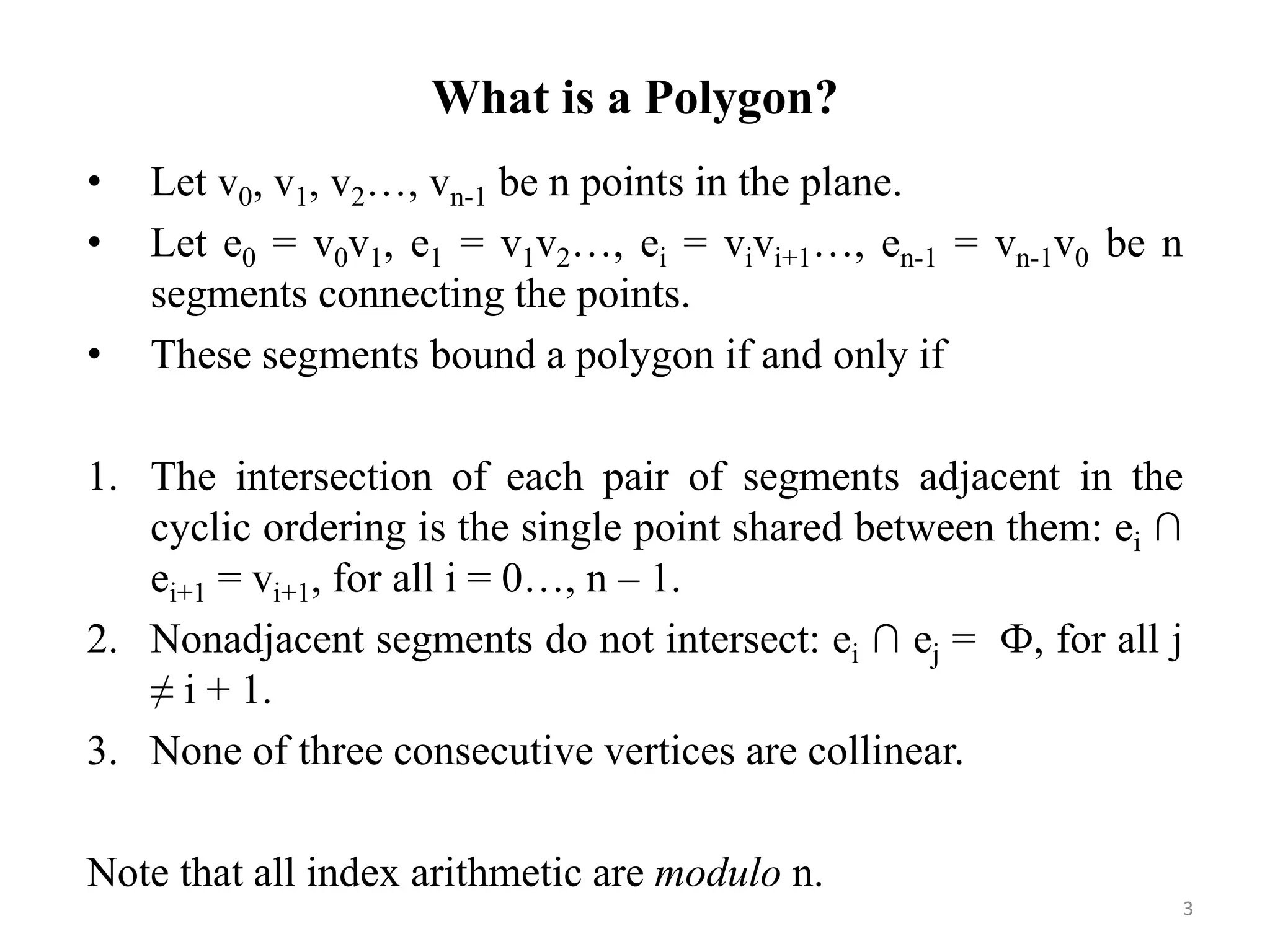
The document presents an algorithm to find the visible region of a polygon in O(n^2) time and O(n) space. It first finds the visible vertices region by checking each vertex for intersections with edges in O(n^2) time. It then extends this region to the full visible region by considering gaps between visible vertices and finding intersection points of extreme lines in O(n) time. The algorithm avoids issues with existing approaches and produces the exact visible region without unnecessary points.


![Assignment for Factory Method Design Pattern in C# [ANSWERS]](https://cdn.slidesharecdn.com/ss_thumbnails/assingment1answers-200420114633-thumbnail.jpg?width=640&height=640&fit=bounds)