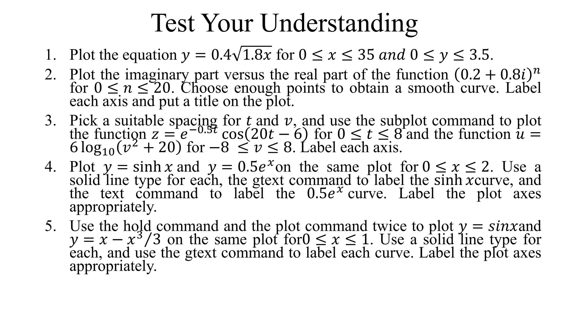
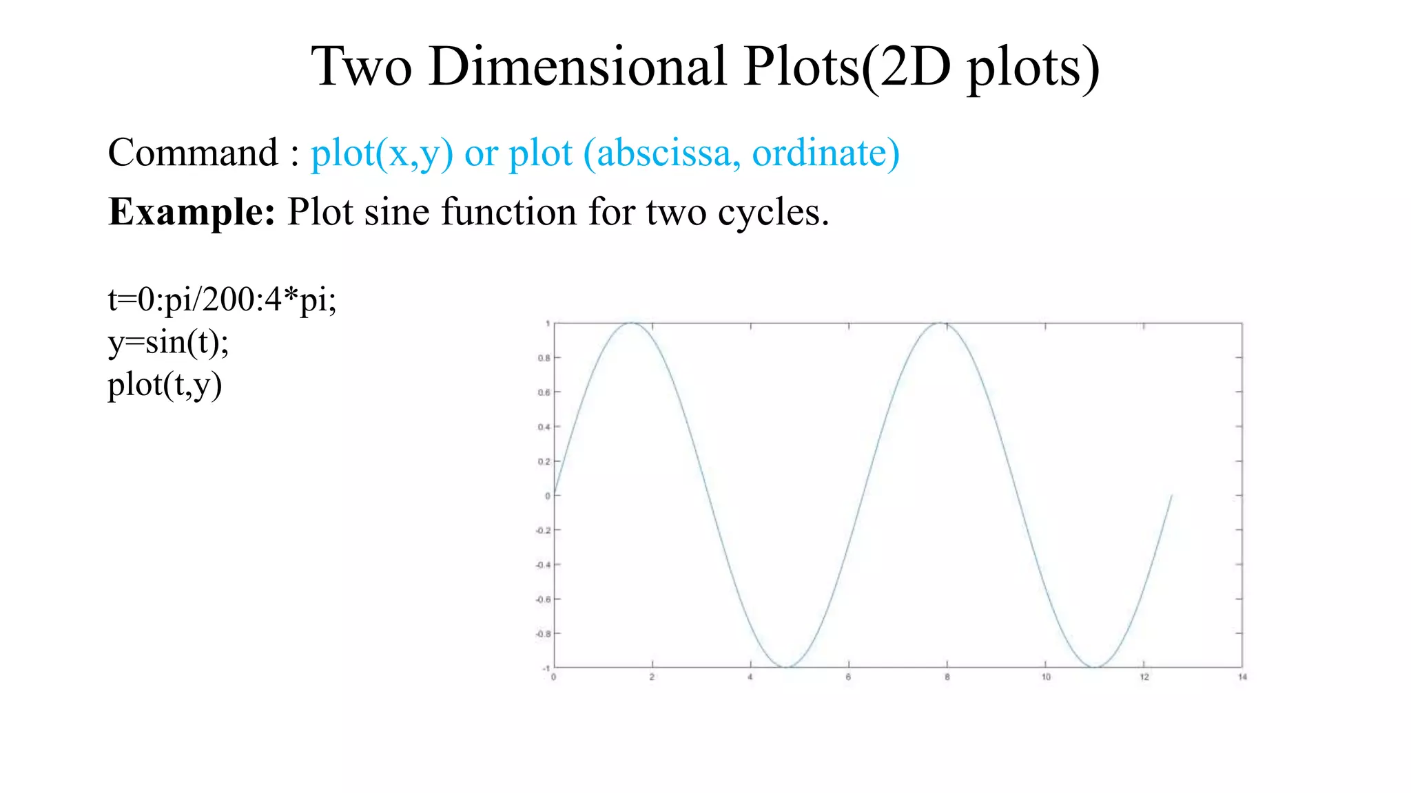
Here are the steps to plot the given functions using MATLAB: 1. Plot y = 0.4x + 1.8 for 0 ≤ x ≤ 35 and 0 ≤ y ≤ 3.5: x = 0:35; y = 0.4.*x + 1.8; plot(x,y) xlim([0 35]) ylim([0 3.5]) 2. Plot imaginary vs real parts of 0.2 + 0.8i*n for 0 ≤ n ≤ 20: n = 0:20; z = 0.2 + 0.8i*n; plot(real(z),imag(z)) xlabel('Real Part')

1. Experiment-2
Trigonometric Function, Complex Numbers & M Files in
MATLAB/ Graph & Plotting in MATLAB
Mr. Kumar Prabhakar
Electronics & Communication Engineering
PDPM
Indian Institute of Information Technology,
Design and Manufacturing Jabalpur

2. Experiment-2
MATLAB Graph & plotting
Overview
• MATLAB has an excellent set of graphic tools.
• Plotting a given data set or the results of computation is possible with
very few commands.
• Understanding of mathematical equations with graphics is an
enjoyable and very efficient way of learning mathematics
• Being able to plot mathematical functions and data freely is the most
important step, and this section is written to assist you to do just that.

3. Two Dimensional Plots(2D plots)
Command : plot(x,y) or plot (abscissa, ordinate)
Example: Plot sine function for two cycles.
t=0:pi/200:4*pi;
y=sin(t);
plot(t,y)

4. Two Dimensional Plots(2D plots)
Adding titles and axis labels: MATLAB also allows labelling of axes.
i.e. x,y axes and title.
Command : xlabel(‘string’)
xlabel() function allows to label the x-axis
Command : ylabel(‘string’)
ylabel() function allows to label the y-axis
Command: title(‘string’)
title()– function allows giving title to our plot.
Note : The order of the xlabel, ylabel, and title commands does not
matter, but we must place them after the plot command.

5. Two Dimensional Plots(2D plots)
Line styles, Markers and Colours:
Various line types, plot symbols and colors may be obtained with
plot(x,y,s) where s is a character string made from one element from any
or all the following 3 columns given below.
Note : Default colour of graph is blue

6. Two Dimensional Plots(2D plots)
Controlling Axes
• The scaling and appearance of plot axis can be controlled with the axis
function. To set scaling for the x and y axes on the current 2-D plot,
use the below given command:
Command: axis([xmin xmax ymin ymax])
• Others use full command for axis controlling are:
Command: axis('auto’); axis('square’) ; axis('off ‘) ; axis(tight);
axis(equal)

7. Two Dimensional Plots(2D plots)
Multiple data sets in one plot
• Many times you may have to plot many functions in different figures
or multiple functions in the same figure. The following piece of code
is an initial attempt to create many plots together.
• For example, these statements plot three related functions of t: y1 = 2*
cos(t), y2 = cos(t), y3 = 0.5 ∗ cos(t), and y4=sin(t) in the interval 0 ≤ t
≤ 2π.
Using single plot command
Using multiple plot commands [hold on hold off]

8. Two Dimensional Plots(2D plots)
Subplotting
• Sometimes creating a single plot for several functions is not practical
due to different scales and units of the functions.
• Science and Engineering applications, often it is desirable to visualize
many functions together, and subplot command can easily serve the
purpose in place of having many different plots and trying to bring
them together.
Example: The average yearly rainfall and production of rice in a
particular state is given by the following table for 7 consecutive years:

9. Two Dimensional Plots(2D plots)
• The subplot command allows you to separate the figure into as many
plots as desired, and arrange them all in one figure.
• The general format of this command is : subplot(m,n,p)

10. Two Dimensional Plots(2D plots)
Create chart with two y-axes
• Command: plotyy(x1,y1,x2,y2)
Produces a plot with two y axes, y1 on the left and y2 on the right
• Command: gtext(‘text’)
Places the string text in the Figure
window at a point specified by the
mouse.

11. Two Dimensional Plots(2D plots)
Create chart with two y-axes
• Command: yyaxis left
yyaxis right

12. Specialized plot commands
Two Dimensional Plots(2D plots)

13. Two Dimensional Plots(2D plots)
Error Bar Plots
Command: errorbar(X,Y,E)
• Experimental data are often represented with plots containing error
bars.
• The bars show the estimated or calculated errors for each data point.
• They can also be used to display the error in an approximate formula.
Example: Keeping two terms in the Taylor series expansion of
𝑐𝑜𝑠𝑥 about 𝑥 = 0 gives 𝑐𝑜𝑠𝑥 ≈ 1 − 𝑥2 2.

14. Two Dimensional Plots(2D plots)
Box plot
Command: boxplot(x)
• boxplot(x) creates a box plot of the data in x. If x is a vector, boxplot
plots one box. If x is a matrix, boxplot plots one box for each column
of x.
• On each box, the central mark indicates the median, and the bottom
and top edges of the box indicate the 25th and 75th percentiles,
respectively.
• The whiskers extend to the most extreme data points not considered
outliers, and the outliers are plotted individually using the '+' marker
symbol.

15. Note: Each box visually represents the MPG data for cars from the specified country. Italy's "box"
appears as a single line because the sample data contains only one observation for this group
Two Dimensional Plots(2D plots)

16. Trigonometry function
• The trigonometric functions in MATLAB calculate standard
trigonometric values in radians or degrees, hyperbolic trigonometric
values in radians, and inverse variants of each function.
• You can use the rad2deg and deg2rad functions to convert between
radians and degrees, or functions like cart2pol to convert between
coordinate systems.
sin Sine of argument in radians
sind Sine of argument in degrees
sinpi Compute sin(X*pi) accurately
asin Inverse sine in radians
asind Inverse sine in degrees
sinh Hyperbolic sine
asinh Inverse hyperbolic sine
cos Cosine of argument in radians
cosd Cosine of argument in degrees
cospi Compute cos(X*pi) accurately
acos Inverse cosine in radians
acosd Inverse cosine in degrees
cosh Hyperbolic cosine
acosh Inverse hyperbolic cosine

17. tan Tangent of argument in radians
tand Tangent of argument in degrees
atan Inverse tangent in radians
atand Inverse tangent in degrees
atan2 Four-quadrant inverse tangent
atan2d Four-quadrant inverse tangent in degrees
tanh Hyperbolic tangent
atanh Inverse hyperbolic tangent
csc Cosecant of input angle in radians
cscd Cosecant of argument in degrees
acsc Inverse cosecant in radians
acscd Inverse cosecant in degrees
csch Hyperbolic cosecant
acsch Inverse hyperbolic cosecant
sec Secant of angle in radians
secd Secant of argument in degrees
asec Inverse secant in radians
asecd Inverse secant in degrees
sech Hyperbolic secant
asech Inverse hyperbolic secant
Trigonometry function

18. Degrees/Radians Conversion and Coordinate
Conversion
Degrees/Radians Conversion
deg2rad Convert angle from degrees to radians
rad2deg Convert angle from radians to degrees
cart2pol Transform Cartesian coordinates to polar or cylindrical
cart2sph Transform Cartesian coordinates to spherical
pol2cart Transform polar or cylindrical coordinates to Cartesian
sph2cart Transform spherical coordinates to Cartesian
Coordinate Conversion

19. Complex Numbers
• In MATLAB, i and j represent the basic imaginary unit. You can use
them to create complex numbers such as 2i+5.
• You can also determine the real and imaginary parts of complex
numbers and compute other common values such as phase and angle.
Basic commands:
abs Absolute value and complex magnitude
angle Phase angle
complex Create complex array
conj Complex conjugate
cplxpair Sort complex numbers into complex conjugate pairs
i Imaginary unit
imag Imaginary part of complex number
isreal Determine whether array uses complex storage
j Imaginary unit
real Real part of complex number

20. Test Your Understanding
1. Plot the equation 𝑦 = 0.4 1.8𝑥 for 0 ≤ 𝑥 ≤ 35 𝑎𝑛𝑑 0 ≤ 𝑦 ≤ 3.5.
2. Plot the imaginary part versus the real part of the function 0.2 + 0.8𝑖 𝑛
for 0 ≤ 𝑛 ≤ 20. Choose enough points to obtain a smooth curve. Label
each axis and put a title on the plot.
3. Pick a suitable spacing for 𝑡 and 𝑣, and use the subplot command to plot
the function 𝑧 = 𝑒−0.5𝑡
cos 20𝑡 − 6 for 0 ≤ 𝑡 ≤ 8 and the function 𝑢 =
6 log10 𝑣2
+ 20 for −8 ≤ 𝑣 ≤ 8. Label each axis.
4. Plot 𝑦 = sinh 𝑥 and 𝑦 = 0.5𝑒𝑥on the same plot for 0 ≤ 𝑥 ≤ 2. Use a
solid line type for each, the gtext command to label the sinh 𝑥curve, and
the text command to label the 0.5𝑒𝑥
curve. Label the plot axes
appropriately.
5. Use the hold command and the plot command twice to plot 𝑦 = 𝑠𝑖𝑛𝑥and
𝑦 = 𝑥 − 𝑥3
3 on the same plot for0 ≤ 𝑥 ≤ 1. Use a solid line type for
each, and use the gtext command to label each curve. Label the plot axes
appropriately.

21. Test Your Understanding