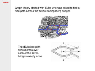
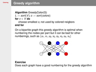
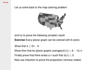
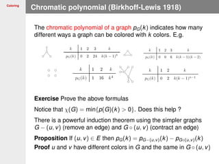
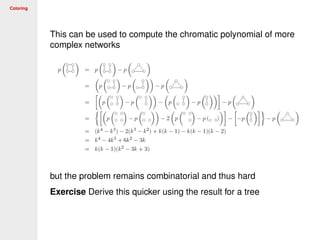
The document provides an overview of graph theory and applications. It begins with a brief history of graph theory starting with Euler and Hamilton. It then summarizes some key graph theory concepts like connectivity, paths, trees, and coloring problems. The document outlines several applications of graph theory including ranking web pages, finding the shortest path with GPS, and analyzing large networks and graphs. It concludes by mentioning some large scale graph problems like similarity of nodes, telephony networks, and clustering large graphs.


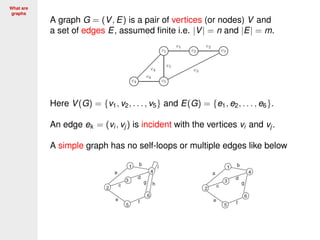
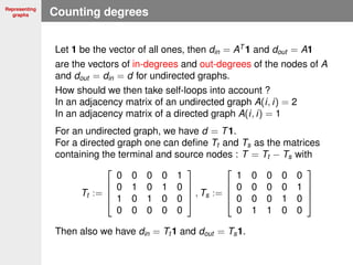
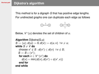
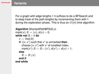
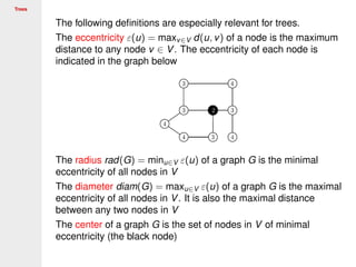
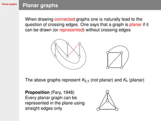
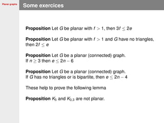
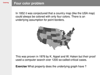
![Complexity
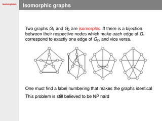
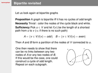
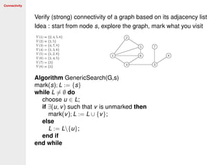
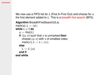
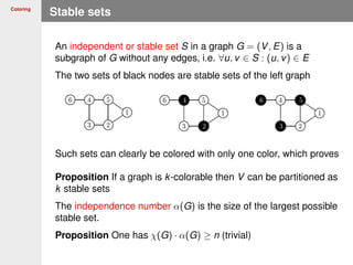
Comparing problems
A problem Y is reducible (in polynomial time) to a problem X if
X is at least as difficult to solve as Y, denoted as X ≥p Y. Then
X ≥p Y and X ∈ P implies Y ∈ P
X ≥p Y and Y /∈ P implies X /∈ P
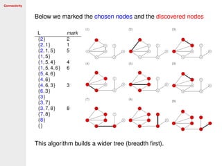
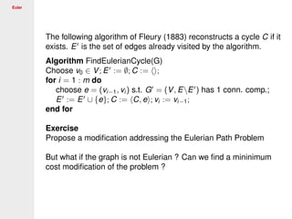
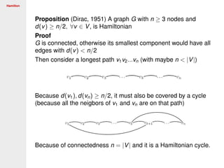
Define the problem [LongestPath(u, v, w, N)] of finding a path
of length ≥ any N from u to v in a graph with integer weights w
Proposition [HamiltonianCycle] ≤p [LongestPath(u, v, w, N)]
Proof Choose unit weights w. Pick an edge e = (u, v).
If there is a longest path of length N = n − 1 in G = Ge,
then G is Hamiltonian. Try out all m < n2
/2 edges.
Since we know that the Hamiltonian cycle problem in not in P
the longest path problem is also not in P.](https://image.slidesharecdn.com/graph-170205092337/85/Graph-106-320.jpg)
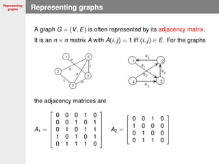
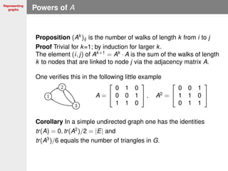
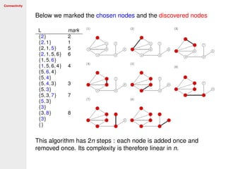
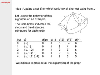
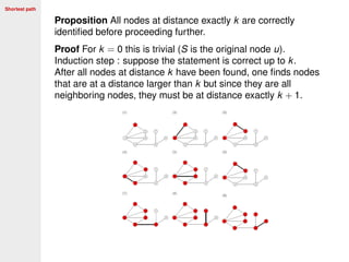
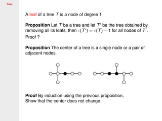
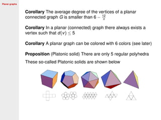
![Complexity
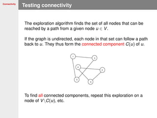
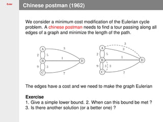
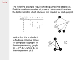
A Boolean clause is a disjunction of Boolean terms Xi ∈ {0, 1} and
their negation Xi ∈ {0, 1}, e.g. X1 ∨ X2 ∨ X4 ∨ X7 is a 4-term.
Define the problem [SAT] as checking if a set of Boolean clauses
can be simultaneously satisfied ([3SAT] involves only 3-terms).
E.g. {X2 ∨ X2, X2 ∨ X3 ∨ X4, X1 ∨ X4} can be satisfied by choosing
X1 = 1, X2 = 0, X3 = 1, X4 = 0.
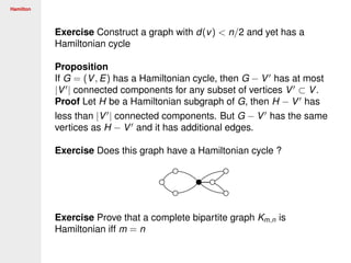
Proposition [SAT] ≤p [3SAT] and [3SAT] ≤p [StableSet]
Proof We do not prove the first part involving only 3-terms.
Construct a triangle for
each 3-term and then
connect the negations
across triangles
For a stable set, I can choose only one node in each triangle.
Then there is a stable set of size n/3 iff [3SAT] is satisfiable.](https://image.slidesharecdn.com/graph-170205092337/85/Graph-107-320.jpg)
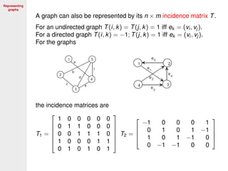
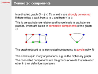
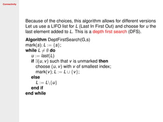
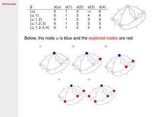
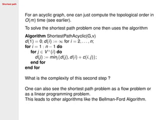
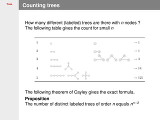
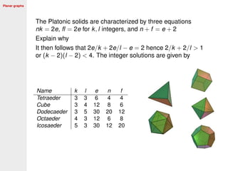
![Complexity
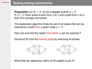
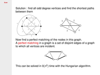
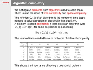
[3SAT] is known to be NP-complete.
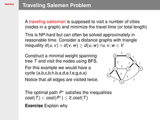
We now prove that also the [CLIQUE] problem is NP-complete
The [CLIQUE] problem is checking if there exists a clique
(complete subgraph) of size k in a graph G = (V, E)
Proof Consider {X1 ∨ X2 ∨ X3, X1 ∨ X2 ∨ X3, X1 ∨ X2 ∨ X3}.
Construct a graph with the terms of each clause as nodes.
Then connect all pairs of variable except their negation (partially
done below)
If this graph contains a clique of size 3, the clause is satisfiable.](https://image.slidesharecdn.com/graph-170205092337/85/Graph-109-320.jpg)