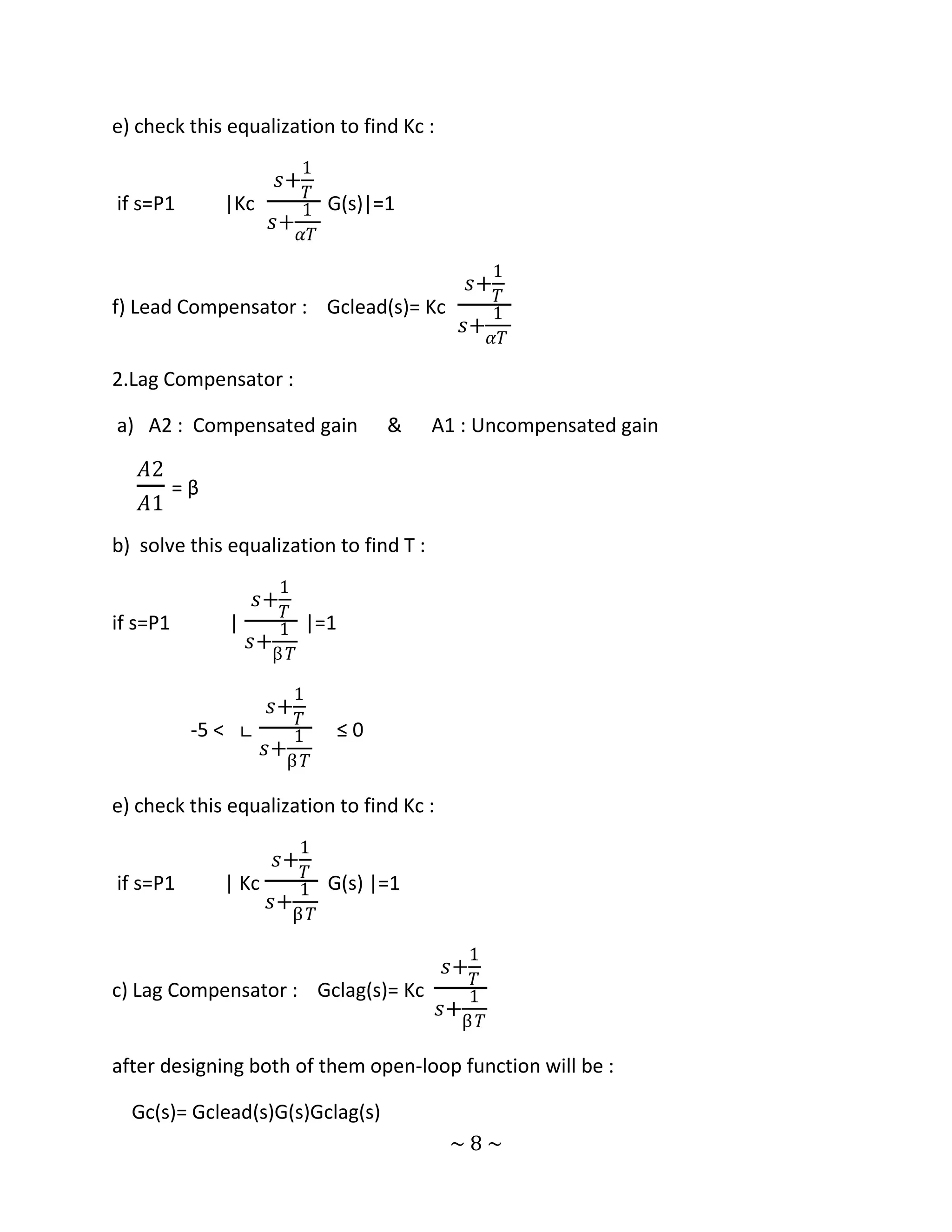
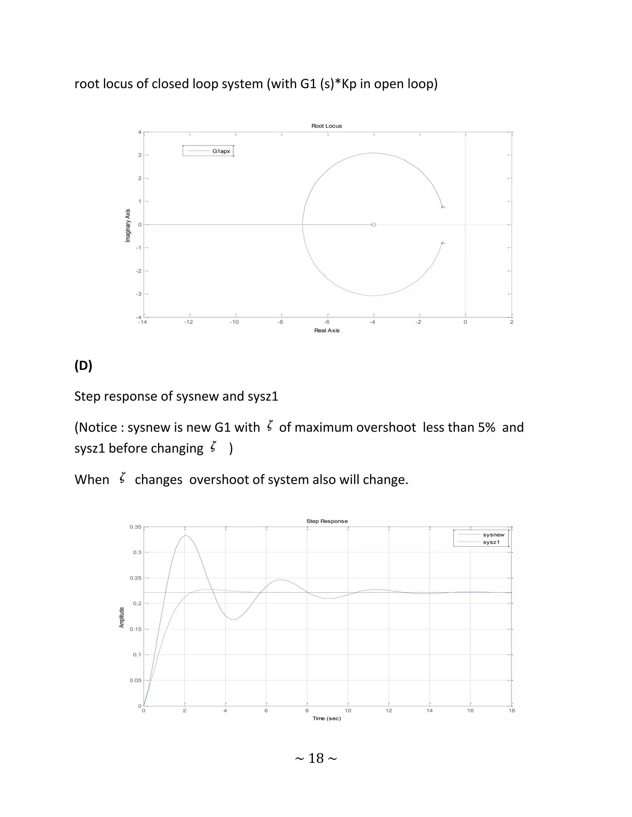
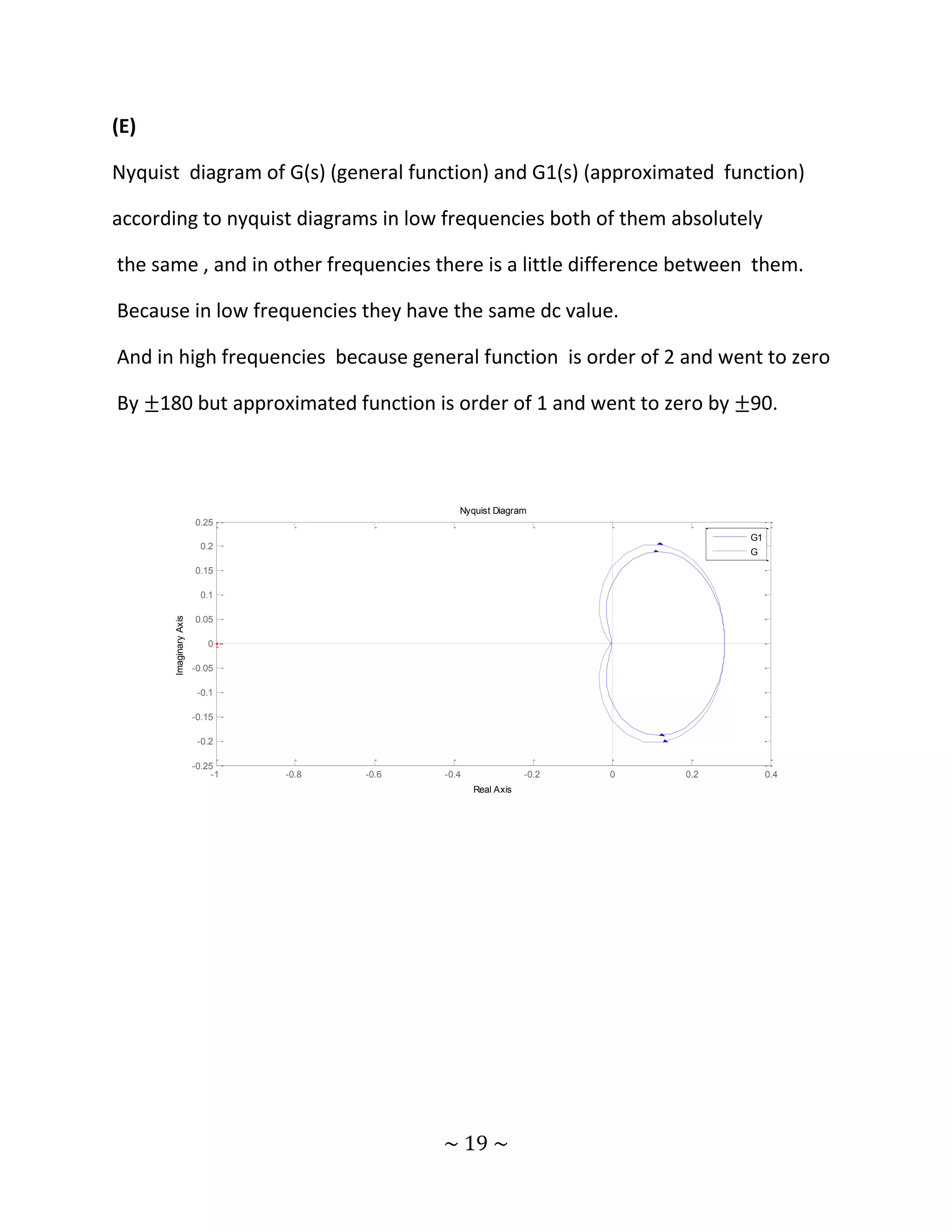
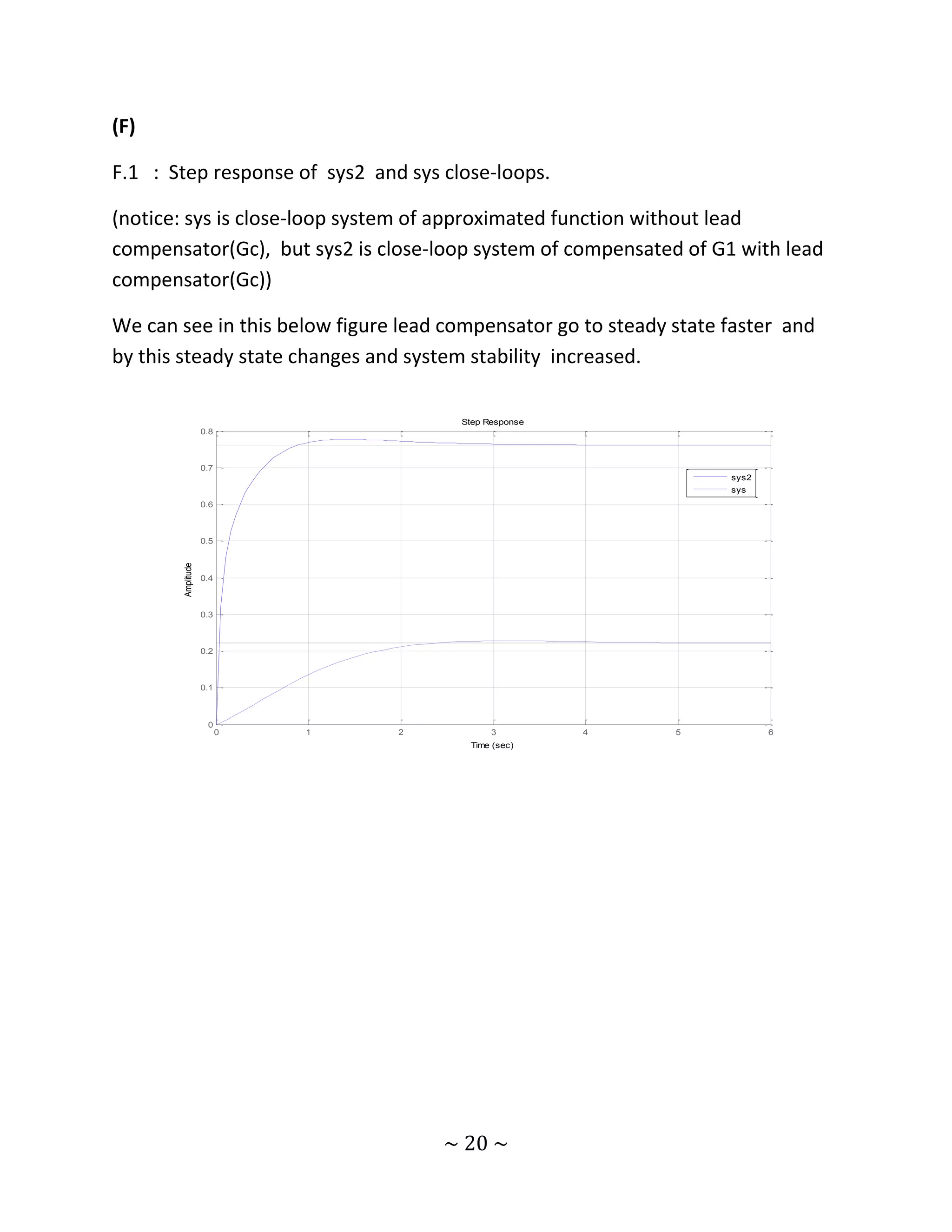
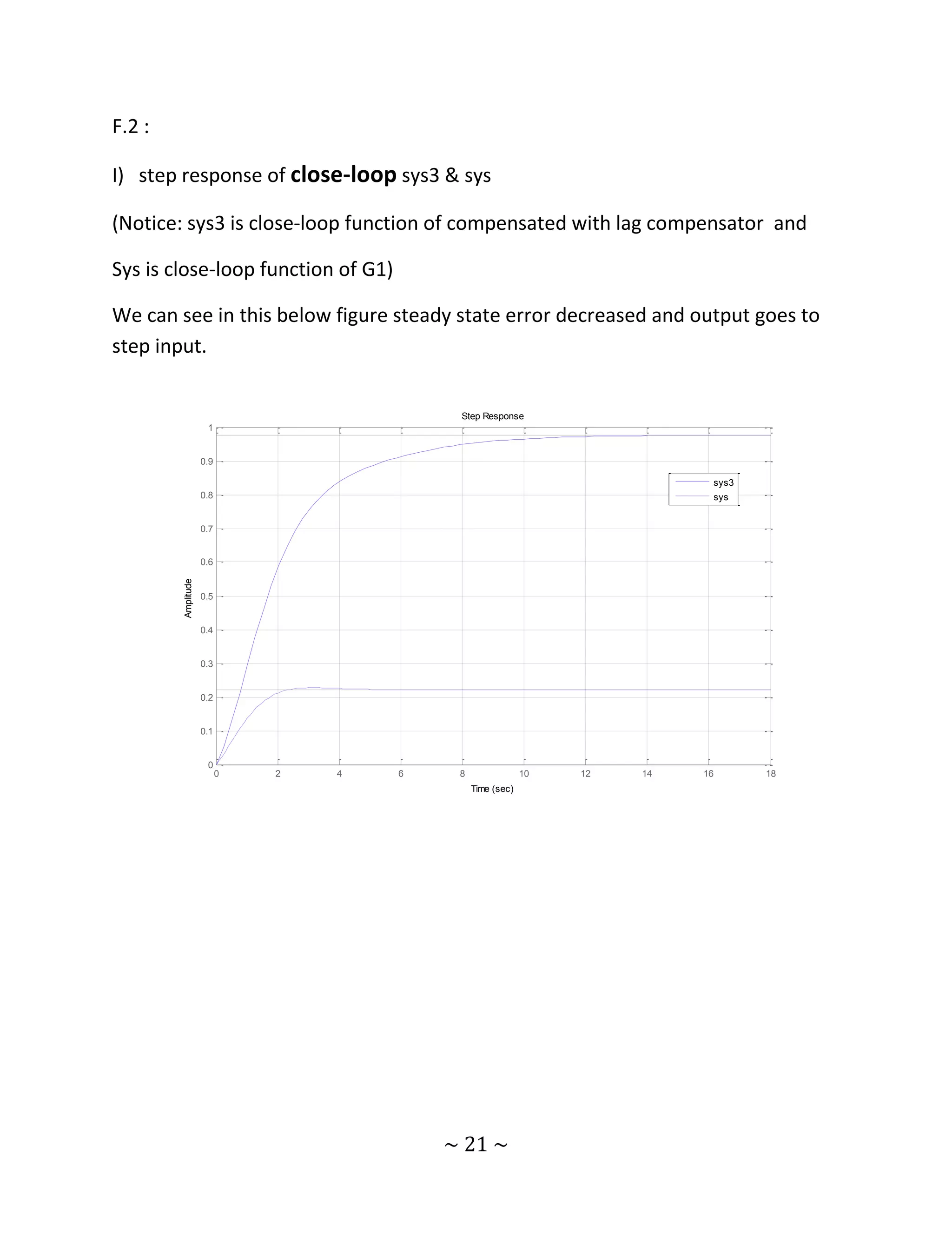
Downloaded 30 times
![Part (G) :
In state space a system defined by this matrixes :
X : state vector (n x 1)
U : input vector (m x 1)
Y : output vector (p x 1)
A : system matrix (n x n)
B : system input matrix (n x m)
C : output matrix (p x n)
D : input matrix ,usually for SISO systems is 0
When this matrixes go into state space :
sX(s)=AX(s)+BU(s)
Y(s)=CX(s)+DU(s)
If these equalization solved :
X(s)=(𝑠𝐼 − 𝐴)−1 BU(s)
G(s)=C(𝑠𝐼 − 𝐴)−1 B+D
Roots of det(𝑠𝐼 − 𝐴 ) will be Poles of G(s) .
We can check controllability of system by this way :
Q=[ B AB 𝐴2 B …… 𝐴 𝑛 −1 B]
If rank(Q)=n : system is controllable
Otherwise : system is uncontrollable
~9~](https://image.slidesharecdn.com/howtodesignalinearcontrolsystem-121223045408-phpapp02/75/How-to-design-a-linear-control-system-9-2048.jpg)
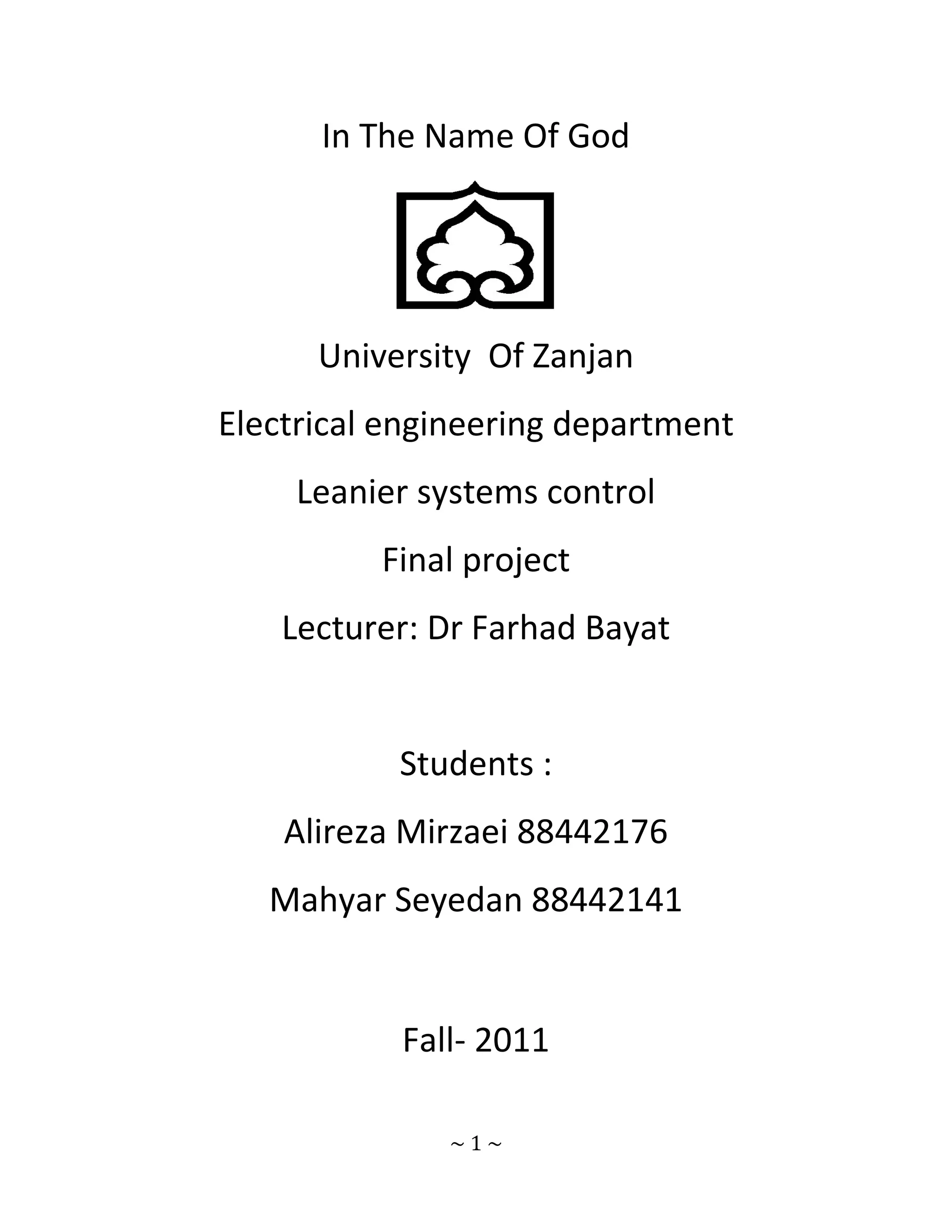
![Simulink by Matlab :
%part A
N=[1 112/25 48/25];
D=[1 23/2 25 93/4 27/4];
G=tf(N,D);
p=pole(G);
z=zero(G);
g=zpk(G);
N1=[1 4];
D1=[1 2 1.5];
k1=polyval(N,0)/polyval(D,0);
k2=polyval(N1,0)/polyval(D1,0);
k3=(k1/k2);
N1=N1*k3;
G1=tf(N1,D1);
g1=zpk(G1);
figure
pzmap(G);
figure
pzmap(G1);
%----------------------------------------------------------
--
%PART B
figure
step(G1,G,'--');
grid;
figure
impulse(G1,G,'--');
grid;
%----------------------------------------------------------
--
%PART C
Kpgeneral=polyval(N,0)/polyval(D,0);
~ 11 ~](https://image.slidesharecdn.com/howtodesignalinearcontrolsystem-121223045408-phpapp02/75/How-to-design-a-linear-control-system-11-2048.jpg)
![G2=Kpgeneral*G;
G2=feedback(G2,1);
Kpapx=polyval(N1,0)/polyval(D1,0);
G1apx=Kpapx*G1;
G1apx=feedback(G1apx,1);
figure
rlocus(G2);
figure
rlocus(G1apx);
[Gm,Pm,Wg,Wp] = margin(G1apx);
%----------------------------------------------------------
-
%PART D
[Nsys,Dsys]=feedback(N1,D1,1,1);
sysz1=tf(Nsys,Dsys);
Wncl=sqrt(Dsys(3));
zitasys=Dsys(2)/(2*Wncl);
zitasysmax=1/abs(9+(pi)^2);
zitasysmax=sqrt(zitasysmax);
Dsys(2)=2*zitasysmax*Wncl;
Nnew=Nsys;
Dnew=Dsys-Nsys;
G1new=tf(Nnew,Dnew);
Kpnew=polyval(Nnew,0)/polyval(Dnew,0);
figure
sysnew=feedback(G1new,1);
step(sysnew,sysz1,'--');
grid;
%----------------------------------------------------------
-
%PART E
figure
nyquist(G1,G,'--');
%----------------------------------------------------------
-
~ 12 ~](https://image.slidesharecdn.com/howtodesignalinearcontrolsystem-121223045408-phpapp02/75/How-to-design-a-linear-control-system-12-2048.jpg)
![%PART F
%F.1(lead compensator)
[numT,denT]= feedback(N1,D1,1,1);
sys=tf(numT,denT);
Wn1=sqrt(denT(3));
Wn2=2*Wn1;
zita1=denT(2)/(2*Wn1);
zita2=zita1;
p1=-(zita2*Wn2)+(Wn2*(sqrt((zita2^2)-1)));
p2=-(zita2*Wn2)-(Wn2*(sqrt((zita2^2)-1)));
p3=pole(sys);
a=p1-p3(1);
b=p1-p3(2);
ph1=pi-angle(a);
ph2=pi-angle(b);
Cph=pi-ph1-ph2;
d=pi-atan(abs((imag(p1))/real(p1)));
m1=tan((Cph+d)/2);
m2=tan((d-Cph)/2);
T=-1/(real(p1)-((imag(p1))/m1));
alpha=-T/(real(p1)-((imag(p1))/m2));
N3=[1 1/T];
D3=[1 1/(alpha*T)];
Gc=tf(N3,D3);
zpk(Gc);
Kc=1/abs((polyval(N3,p1)/polyval(D3,p1))*(polyval(N1,p1)/po
lyval(D1,p1)));
Gc=Kc*Gc;
Gcc=G1*Gc;
sys2=feedback(Gcc,1);
figure
step(sys2,sys,'--');
grid;
%F.2(lag compensator)
Kp1=polyval(N1,0)/polyval(D1,0);
Kp2=100*Kp1;
beta=Kp2/Kp1;
T2=(1-(1/(beta^2))/(-2*real(p1)*(1-(1/beta))));
N4=[1 1/T2];
D4=[1 1/(beta*T2)];
~ 13 ~](https://image.slidesharecdn.com/howtodesignalinearcontrolsystem-121223045408-phpapp02/75/How-to-design-a-linear-control-system-13-2048.jpg)
![Gc2=tf(N4,D4);
zpk(Gc2);
Kc2=1/abs((polyval(N4,p3(1))/polyval(D4,p3(1)))*(polyval(N1
,p3(1))/polyval(D1,p3(1))));
Gc2=Kc2*Gc2;
Gcclag=Gc2*G1;
figure
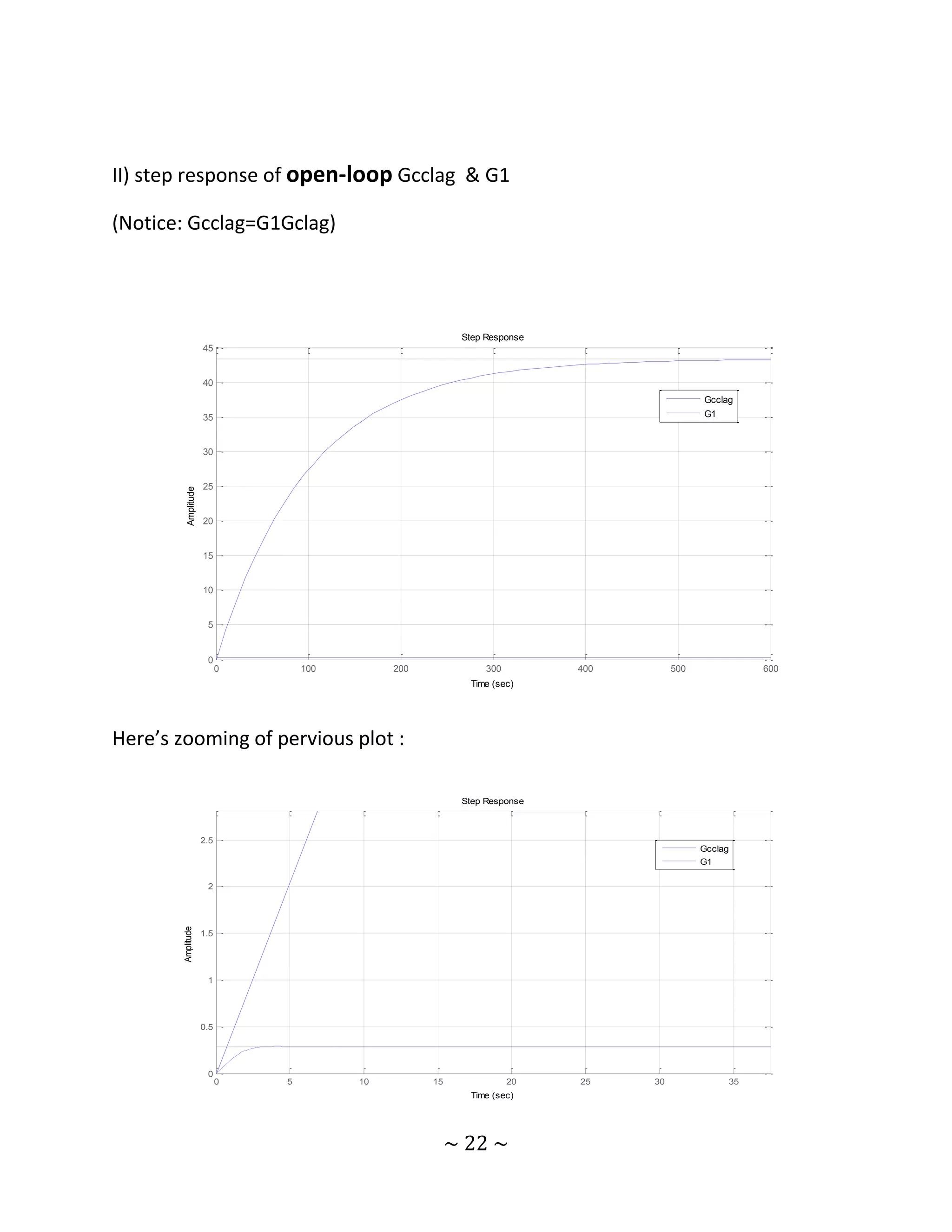
step(Gcclag,G1,'--');
grid;
sys3=feedback(Gcclag,1);
figure
step(sys3,sys,'--');
grid;
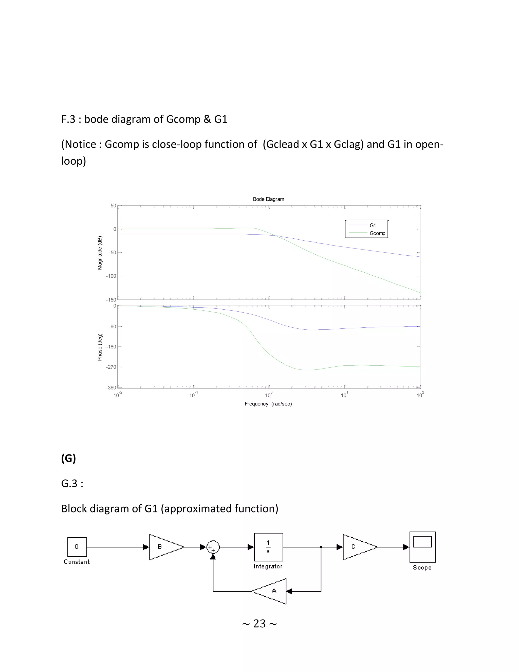
%F.3 Bode diagram
Gcomp=Gcc*G1*Gcclag;
Gcomp=feedback(Gcomp,1);
figure
bode(G1,Gcomp);
%----------------------------------------------------------
-
%PART G
%G FIND A,B,C,D STATE MATRIXS
[NF,DF]=feedback(N1,D1,1,1);
[A,B,C,D]=tf2ss(NF,DF);
%G.1 controlability check
Q=[B A*B ];
r=rank(Q);
disp(r);
%G.2
s=roots(poly(A));
s0=s(1);
s1=s(2);
%G.3 simulinked by matlab (g3.mdl in directory)
~ 14 ~](https://image.slidesharecdn.com/howtodesignalinearcontrolsystem-121223045408-phpapp02/75/How-to-design-a-linear-control-system-14-2048.jpg)
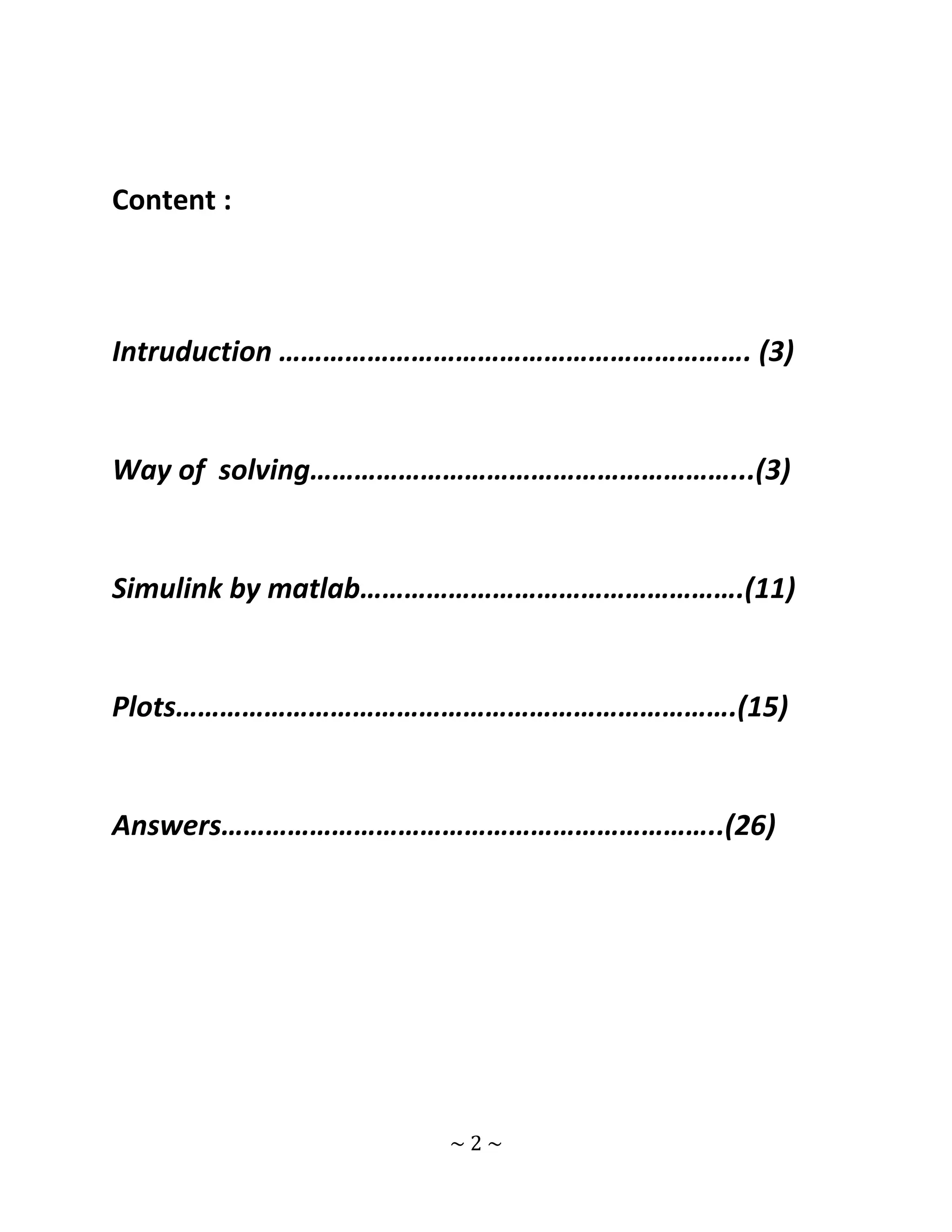
![%G.4
sc1=2*s0;
sc2=4*s1;
J=[sc1 sc2];
K12=acker(A,B,J);
eig(A-B*K12);
disp(K12);
%G.5 simulinked by matlab (g5.mdl in directory)
sysg=ss(A-B*K12,eye(2),eye(2),eye(2));
t=0:0.01:4;
x=initial(sysg,[2;5],t);
x1=[2 5]*x';
x2=[5 2]*x';
figure
subplot(2,1,1);
plot(t,x1),grid;
subplot(2,1,2);
plot(t,x2),grid
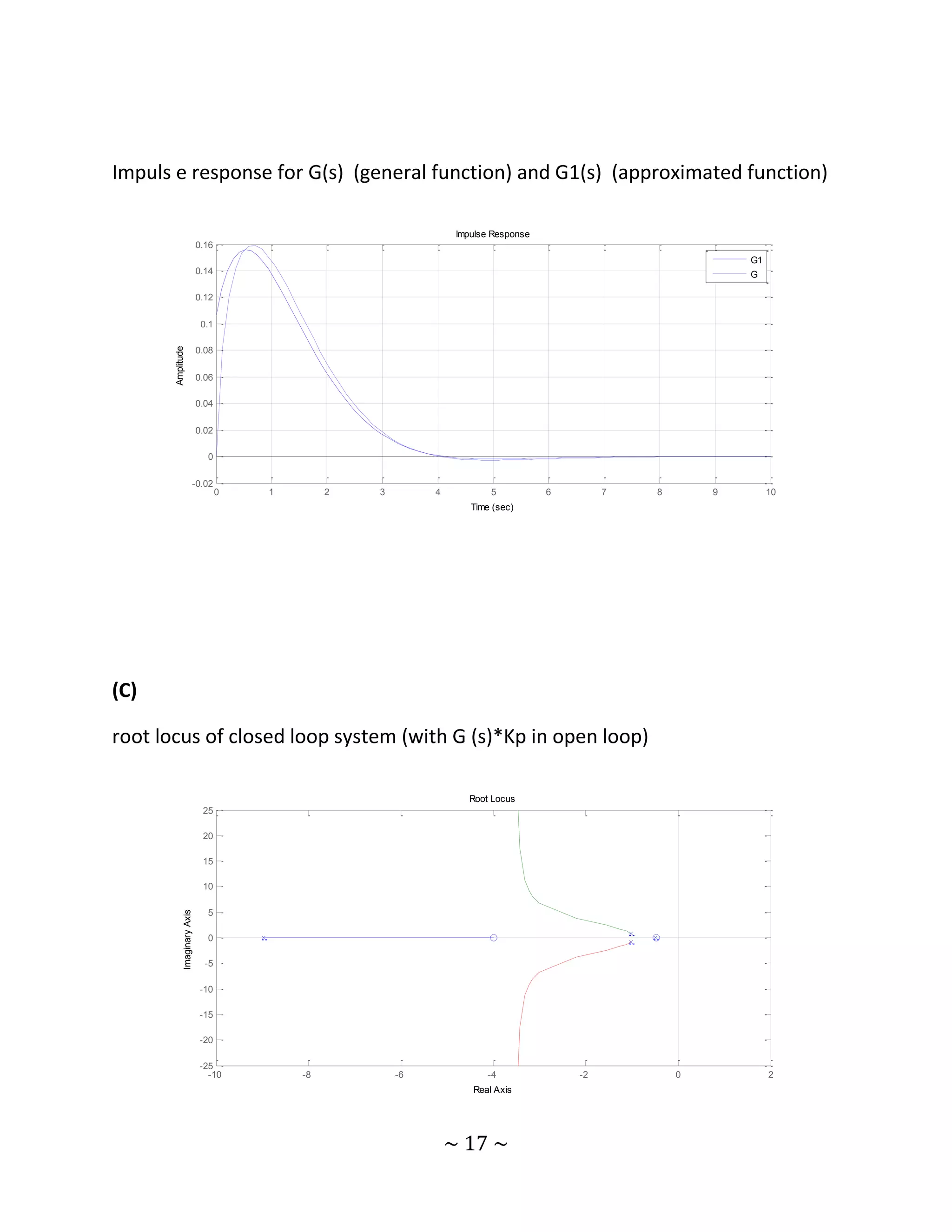
Plots :
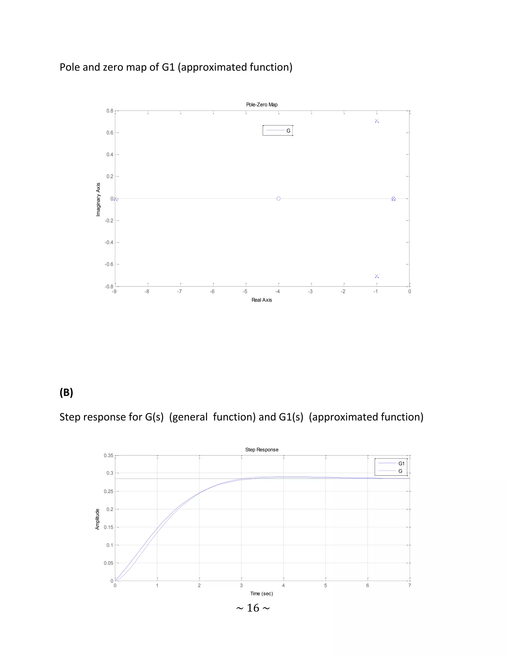
(A)
Pole zero map of G (general function)
Pole-Zero Map
0.8
0.6 G
0.4
0.2
Imaginary Axis
0
-0.2
-0.4
-0.6
-0.8
-9 -8 -7 -6 -5 -4 -3 -2 -1 0
Real Axis
~ 15 ~](https://image.slidesharecdn.com/howtodesignalinearcontrolsystem-121223045408-phpapp02/75/How-to-design-a-linear-control-system-15-2048.jpg)
![initial condition of [2 5] 𝑇 (output of scope in simulink section of Matlab)
G.5 :
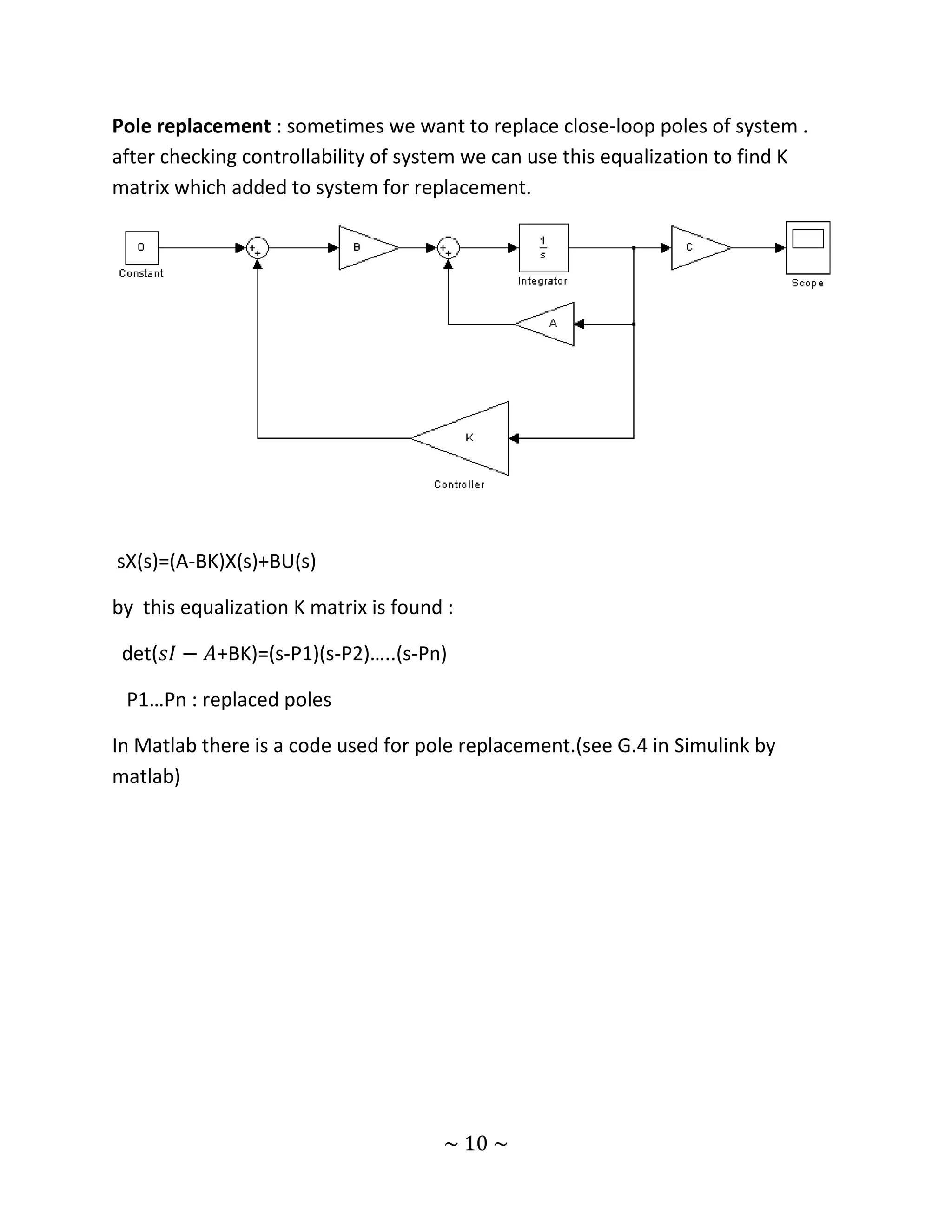
Block diagram of pole replaced system of G1 :
~ 24 ~](https://image.slidesharecdn.com/howtodesignalinearcontrolsystem-121223045408-phpapp02/75/How-to-design-a-linear-control-system-24-2048.jpg)
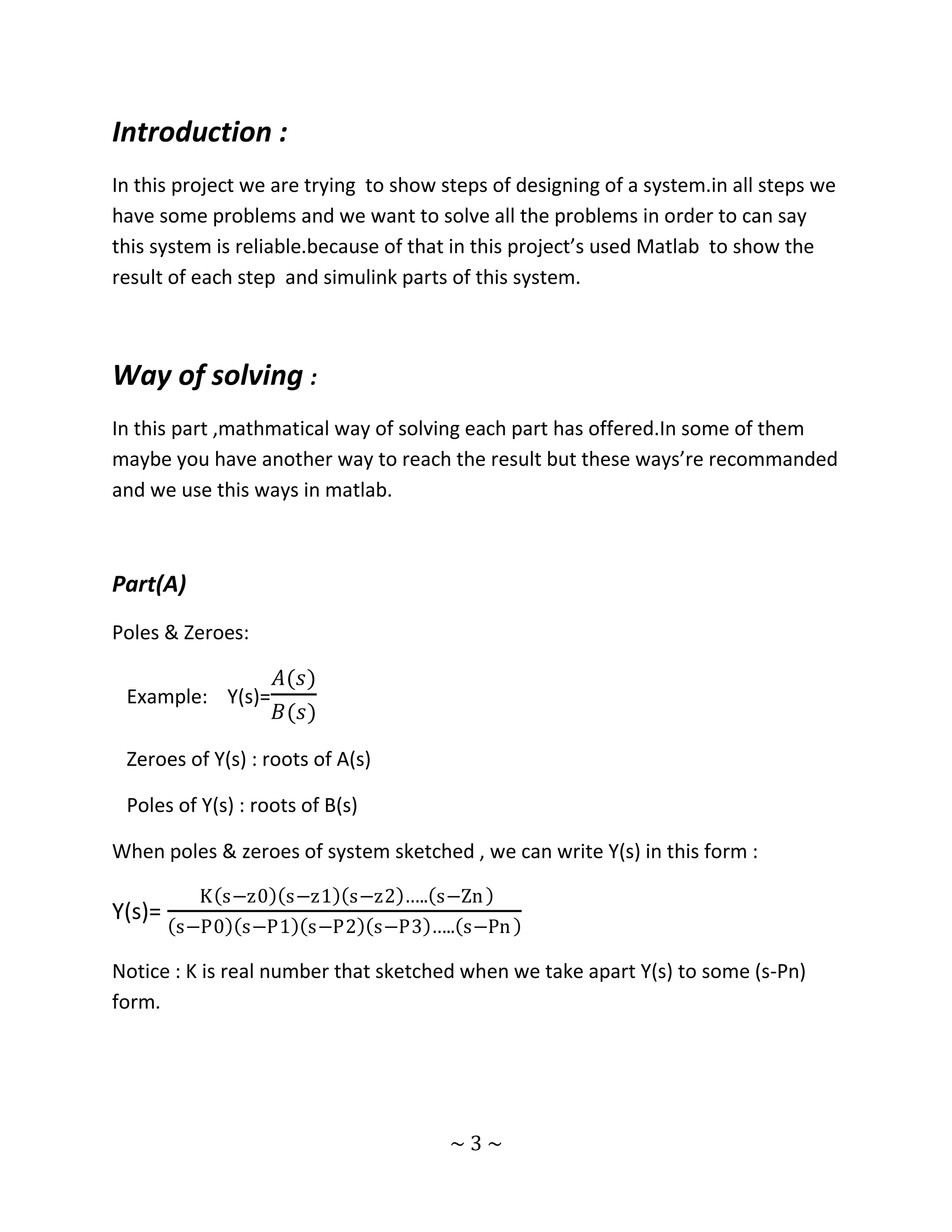
![initial condition of [2 5] 𝑇
I) outputs by M-file section in Matlab in different periods of time
30
20
10
0
-10
0 0.5 1 1.5 2 2.5 3 3.5 4
20
10
0
-10
-20
-30
-40
0 0.5 1 1.5 2 2.5 3 3.5 4
II) output of scope in simulink section of Matlab
~ 25 ~](https://image.slidesharecdn.com/howtodesignalinearcontrolsystem-121223045408-phpapp02/75/How-to-design-a-linear-control-system-25-2048.jpg)
![(Frequency Analysis)
Answers :
F.1 :
165.7 s + 786.8
Gclead(s)=
s + 36.59
F.2 :
0.1626 𝑠 2 + 0.8131 s + 0.6505
Gclag(s)=
𝑠 3 + 2.01 𝑠 2 + 1.52 s + 0.015
F.3 :
0.3066 𝑠 5 + 5.441 𝑠 4 + 37.32 𝑠 3 + 121.7 𝑠 2 + 182.7 s + 93.17
Gctotal(s)= 𝑠8 + 42.6 𝑠7 + 236.5 𝑠6 + 632.5 𝑠5 + 987.9 𝑠4 + 966.3 𝑠3 + 628.3 𝑠2 + 311.1 s+ 94.41
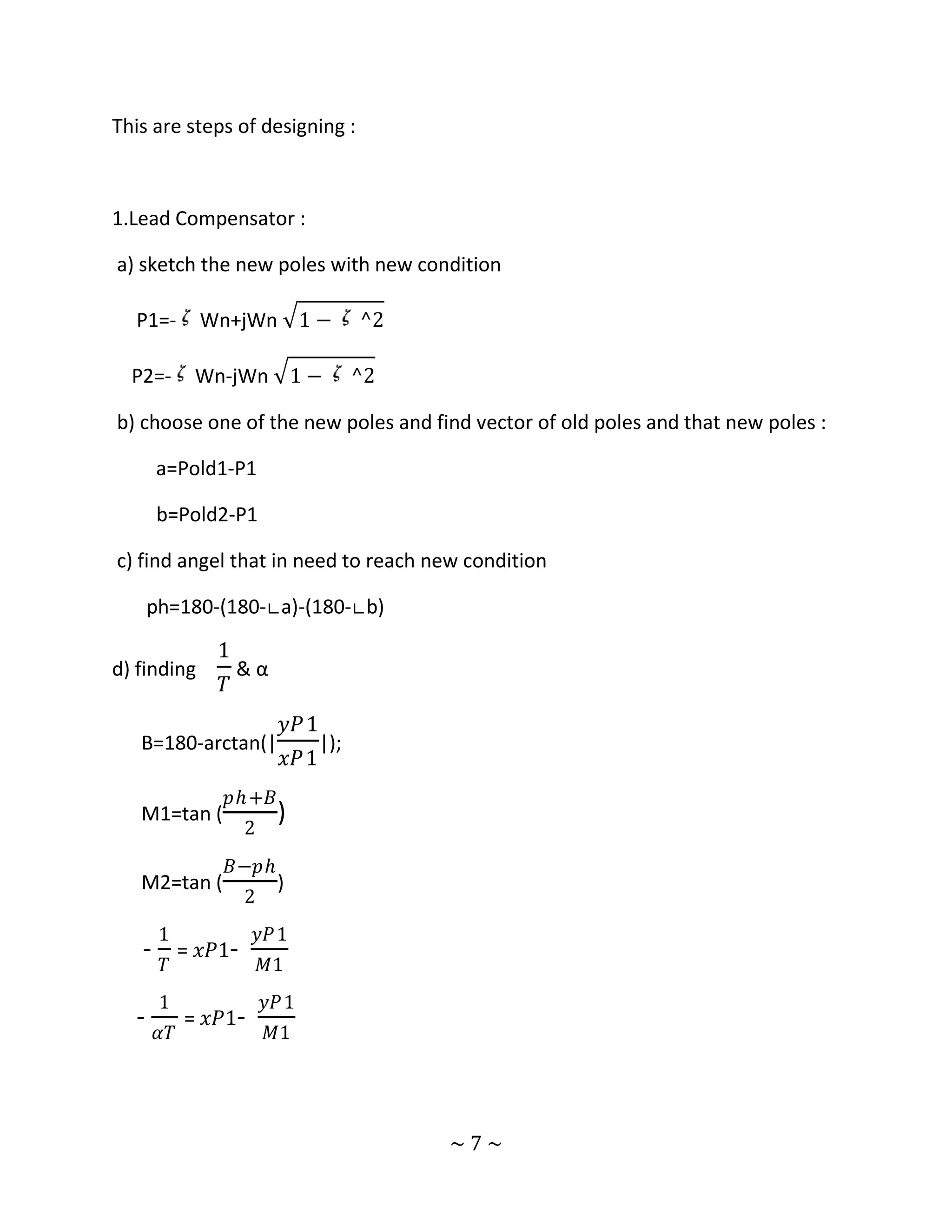
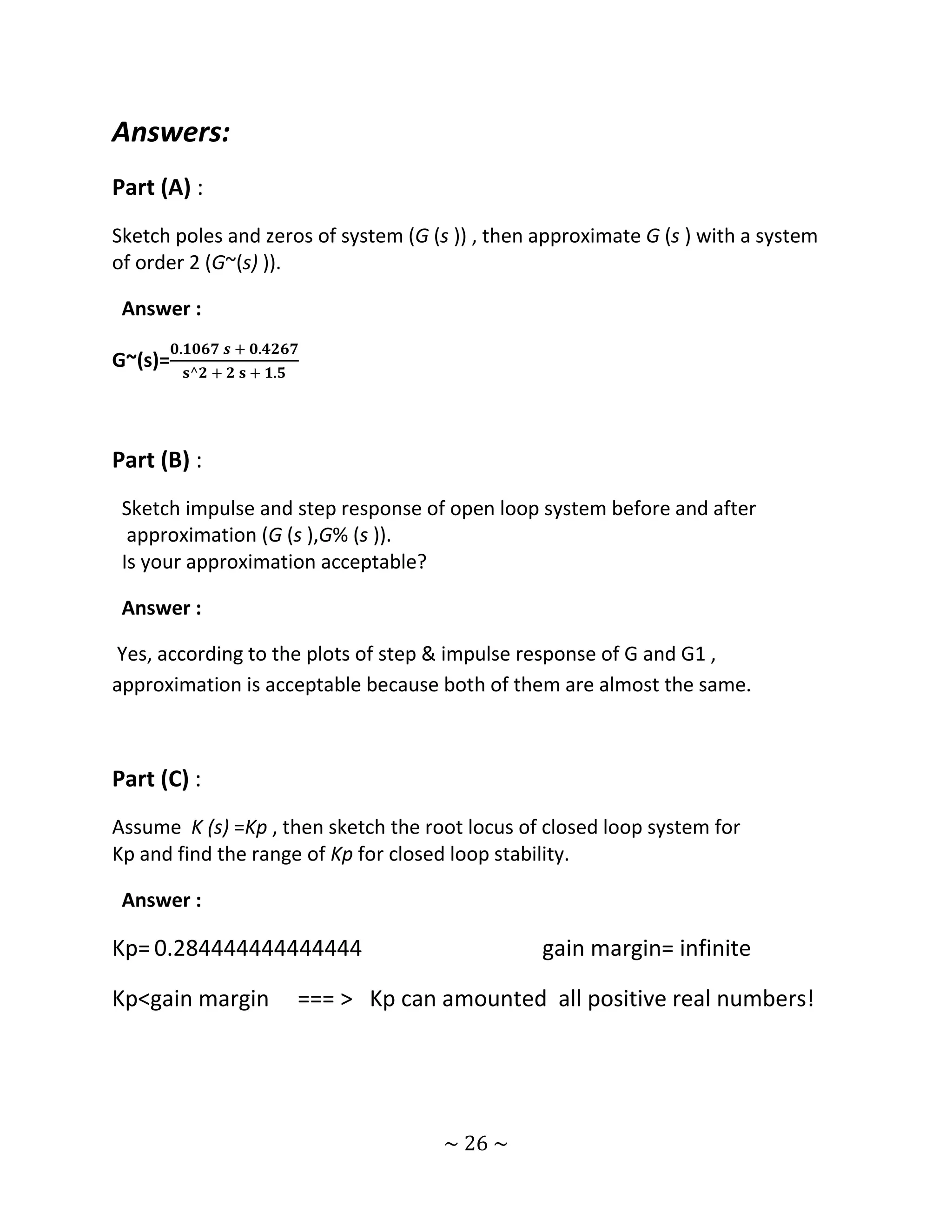
Part (G) :
Find a state space model (A,B ,C ,D ) for approximated
system(G~ (s)
G.1- Check the controllability of system (A,B ,C ,D ) .
G.2- Find all poles of open loop system (So1,So2 by solving det (sI -A) = 0 .
G.3- Sketch the initial condition response of open loop system forX0= [ 2 5 ] 𝑇
G.4- Let U= K.x where K=[K1 K2] , design K1 K2 such that the poles of closed loop
system place at Sc1=2So1 ,Sc2=4So2
~ 28 ~](https://image.slidesharecdn.com/howtodesignalinearcontrolsystem-121223045408-phpapp02/75/How-to-design-a-linear-control-system-28-2048.jpg)
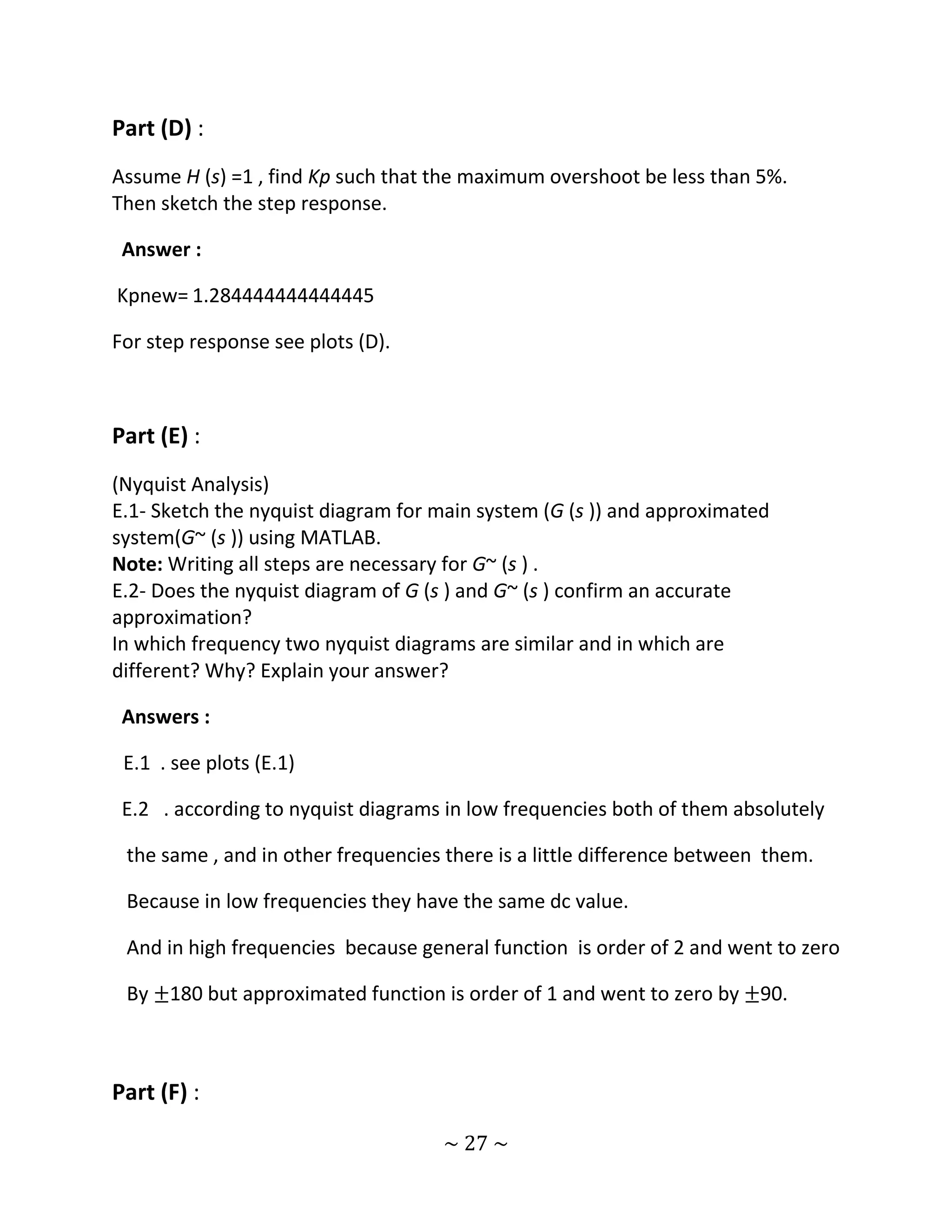
![G.5- Sketch the initial condition response of close loop system forX0= [2 5 ] 𝑇 .
Answers :
G.
−1.926666666666667 −1.926666666666667
A=
1 0
1
B=
0
C= [0.106666666666667 0.426666666666667]
D=0
G.1
Rank(Q)=2 and n=2 ==== > system is controllable!
G.2
So1= -1.053333333333333 + 0.903966567720044i
So2= -1.053333333333333 - 0.903966567720044i
G.3
~ 29 ~](https://image.slidesharecdn.com/howtodesignalinearcontrolsystem-121223045408-phpapp02/75/How-to-design-a-linear-control-system-29-2048.jpg)
![See plots G.3
see and run g3.mdl in project directory
G.4
K=[K1 K2]= [4.213333333333333 13.486666666666668]
G.5
See plots G.5
see and run g5.mdl in project directory
THE END…………………………………………………………………………………………..
~ 30 ~](https://image.slidesharecdn.com/howtodesignalinearcontrolsystem-121223045408-phpapp02/75/How-to-design-a-linear-control-system-30-2048.jpg)

The document presents a detailed final project report from the University of Zanjan's Electrical Engineering Department focused on designing a control system using MATLAB and Simulink. It covers various aspects such as mathematical problem-solving, system response analysis, compensator design, and state-space representation, followed by detailed MATLAB code for simulations. The report includes numerous plots, like pole-zero maps and response graphs, to illustrate results and validate the effectiveness of the proposed control solutions.

![Reduction of multiple subsystem [compatibility mode]](https://cdn.slidesharecdn.com/ss_thumbnails/reductionofmultiplesubsystemcompatibilitymode-110418075355-phpapp01-thumbnail.jpg?width=640&height=640&fit=bounds)


![[ABDO] Data Integration](https://cdn.slidesharecdn.com/ss_thumbnails/dataintegration-1232531198117886-2-thumbnail.jpg?width=640&height=640&fit=bounds)


![[DSBW Spring 2010] Unit 10: XML and Web And beyond](https://cdn.slidesharecdn.com/ss_thumbnails/dsbw-spring-2010-unit-10-xml-and-web-and-beyond3626-thumbnail.jpg?width=640&height=640&fit=bounds)