A System of Estimators of the Population Mean under Two-Phase Sampling in Presence of Two Auxiliary Variables

A System of Estimators of the Population Mean under Two-Phase Sampling in Presence of Two Auxiliary Variables
A System of Estimators of the Population Mean under Two-
Phase Sampling in Presence of Two Auxiliary Variables
1P. A. Patel, *2F. H. Shah
1,2Department of Statistics, Sardar Patel University, Vallabh Vidyanagar 388 120, India
*Corresponding Author: Ms. Fagun Shah, Department of Statistics, Sardar Patel University, Vallabh Vidyanagar 388 120, India.
Email: shah_fagun@yahoo.co.in , Tel: +919712132255; Co-Author Email: patelpraful_a@yahoo.co.in, Tel: +919904494028
This paper deals with estimation of the population mean under two-phase sampling. Utilizing
information on two-auxiliary variables, a system of estimators for estimating the finite population
mean is proposed and its properties, up to the first order of approximation, are studied. As
particular cases various estimators are suggested. The performance of suggested estimators is
compared with some contemporary estimators of the population mean through numerical
illustrations carried over the data set of some natural populations. Also, a small-scale Monte Carlo
simulation is carried out for the empirical comparison.
Keywords: Auxiliary variables, Monte Carlo simulation, Two-phase sampling,
AMS Subject Classification: 62D05; 65C05; 68U20
INTRODUCTION
Auxiliary information on two variables in two-phase sampling has been widely used at estimation stage in order to inflate
the precision of the estimator. For the ordinary ratio and regression estimators of 𝑌, the mean 𝑋 of the auxiliary variable
is estimated by the mean 𝑥′ of the first sample. In single-phase sampling, assuming the linear relationship passes through
origin between 𝑦 and 𝑥, many authors have suggested various estimators of 𝑌 using some known parameters of x such
as mean (𝑋), standard deviation (𝜎𝑥), coefficient of variation (𝐶 𝑥), skewness (𝛽1(𝑥)), kurtosis (𝛽2(𝑥)) and correlation
coefficient (𝜌 𝑦𝑥). For instance, see Upadhyaya and Singh (1999), Singh and Tailor (2003), Kadilar and Cingi (2006),
Khoshnevisan et al. (2007) and references cited in these papers. More often, extra auxiliary variable 𝑧 closely related to
𝑥 but compared to 𝑥 remotely related to 𝑦 is available. For example, 𝑥 is area under the crop wheat in 1964 and 𝑧 is area
under the crop wheat in 1960 (i.e. 𝜌 𝑦𝑧 < 𝜌 𝑥𝑧). In such situations, various estimators were proposed by Chand (1975),
Kiregyera (1980, 1984), Srivenkataramana and Tracy (1989), Srivastava et al. (1990), Sahoo and Sahoo (1993) and
Mishra and Rout (1997), Singh (2008), Hanif (2009), Dash and Mishra (2011), Vishvakarma and Kumar (2014), Ahmed
(2015), Patel and Shah (2018a, b) using two auxiliary variables. Khan (2016, 2017) used single as well as double sampling
scheme to estimate the population mean using two auxiliary variables. Implementing predictive approach, Banopadhyay
and Singh (2016) presented some classes of estimators in the presence of two auxiliary variables under two-phase
sampling design. Motivated from these manuscripts, we seek to estimate the population mean 𝑌 incorporating information
on 𝑥 and 𝑧 at the estimation stage, using two-stage sampling design and suggest a system of estimators which include
many known and unknown estimators.
The present paper introduces a system of estimators for estimating the finite population mean, incorporating partial
auxiliary information on one variable and complete auxiliary information on second variable under two-phase sampling.
This paper is outlined as follows. In next section estimators available in the literature are reviewed. Also, a system of
estimators is proposed and its special cases are discussed. Up to the first order of approximation, bias and MSE are
derived in Section 3. Numerical and empirical studies are carried out in Section 4. Finally, conclusion is presented in
Section 5.
Research Article
Vol. 6(2), pp. 130-136, May, 2019. © www.premierpublishers.org. ISSN: 2375-0499
International Journal of Statistics and Mathematics

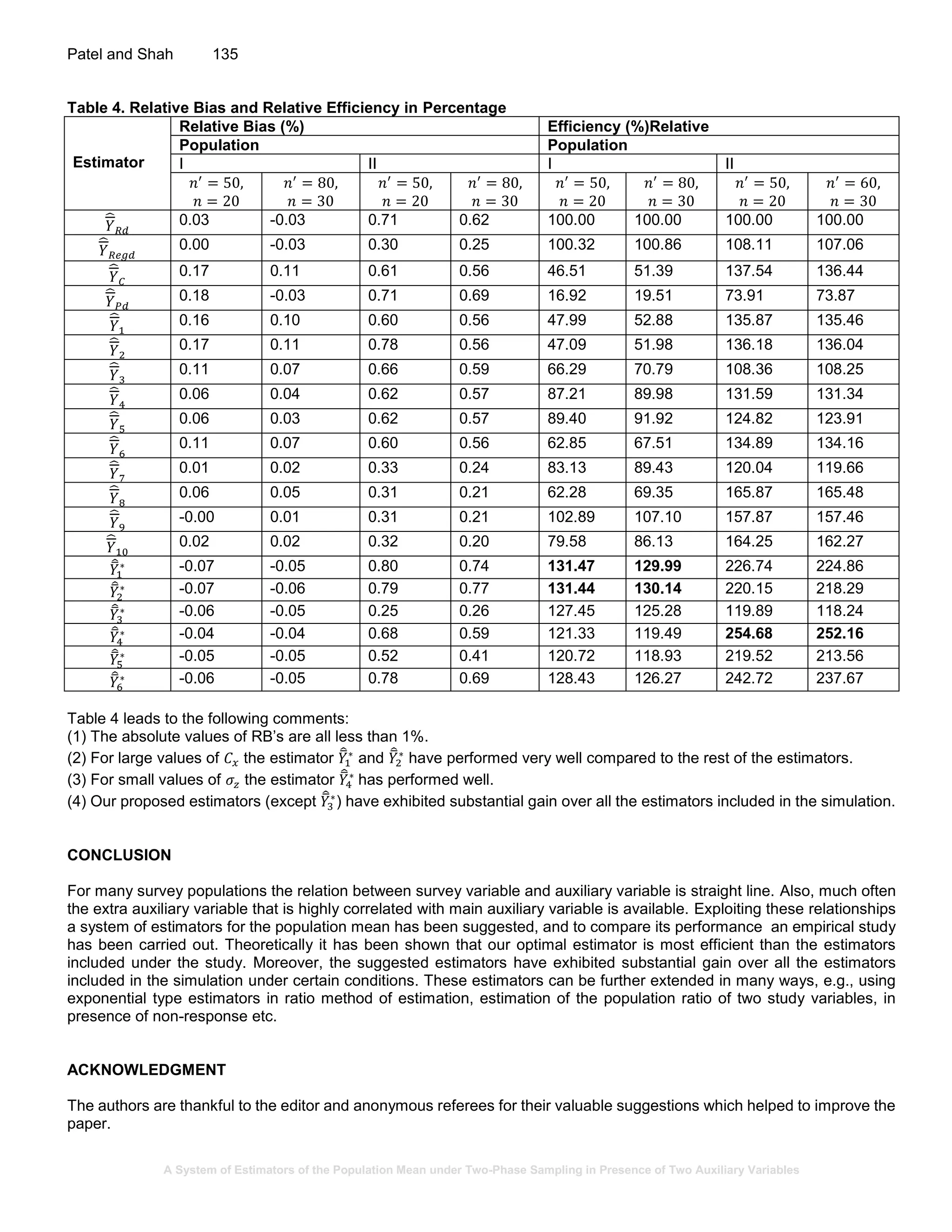
Patel and Shah 131
Existing and Suggested System of Estimators
Consider a two-phase sampling in which a random sample 𝑠′of size 𝑛′ is drawn from the population using simple random
sampling without replacement (SRSWOR) and a subsample 𝑠 of size 𝑛 is drawn using the same sampling design.
Consider a triplet (𝑦𝑖, 𝑥𝑖, 𝑧𝑖) for finite population unit 𝑖 of (1,2, … 𝑁) units where 𝑦𝑖 is the value of the study variable 𝑦 and
𝑥𝑖 and 𝑧𝑖 are the values of auxiliary variables 𝑥 and 𝑧. Here, auxiliary variables 𝑥 > 0 and 𝑧 > 0 are positively correlated
with 𝑦.
Motivated from Khoshnevisan et al. (2007), in this paper we propose a system of estimators for estimating the mean 𝑌
under two-phase sampling that makes use of auxiliary information on two variables at estimation stage. The proposed
system is defined by
𝑌̅̂∗
= 𝑦̅ + 𝑏 𝑦𝑥 [𝑥′ {
𝑎𝑍̅ + 𝑏
𝜆(𝑎𝑧′ + 𝑏) + (1 − 𝜆)(𝑎𝑍̅ + 𝑏)
}
𝐽
− 𝑥] (1)
where 𝑎, 𝑏 and 𝐽 are either real numbers or the functions of the known parameters of the auxiliary variable 𝑧 such as 𝑍,
𝜎𝑧, 𝛽1(𝑧), 𝛽2(𝑧) and 𝜆 ∈ [0, 1] is to be determined so that the system has minimum MSE. This class of estimators include
the following estimators with suitable choice of 𝑎, b, 𝐽 and 𝜆.
Table 1. Members of the System
Estimator Suggested by
Choice of
(𝒂, 𝒃, 𝑱, 𝝀, 𝒃 𝒚𝒙)
𝑌̂
𝑅𝑑 =
𝑦
𝑥
𝑥′ Cochran (1977) (𝑎, 𝑏, 0, 𝜆, 𝑦 𝑥⁄ )
𝑌̂
𝑅𝑒𝑔𝑑 = 𝑦 + 𝑏 𝑦𝑥[𝑥′ − 𝑥] Cochran (1977) (𝑎, 𝑏, 0, 1, 𝑏 𝑦𝑥)
𝑌̂
𝐶 =
𝑦
𝑥
∙
𝑥′
𝑧′
∙ 𝑍 Chand (1975) (1, 0, 1, 1, 𝑦 𝑥⁄ )
𝑌̂
𝑃𝑑 =
𝑦
𝑥
∙ 𝑥′ ∙
𝑧′
𝑍
- (1, 0, −1, 1, 𝑦 𝑥⁄ )
𝑌̂
1 = 𝑦 (
𝑥′
𝑥
) (
𝑍+𝐶 𝑧
𝑧′+𝐶 𝑧
) Singh and Upadhyaya (1995) (1, 𝐶𝑧, 1, 1, 𝑦 𝑥⁄ )
𝑌̂
2 = 𝑦 (
𝑥′
𝑥
) (
𝛽2(𝑧)𝑍+𝐶 𝑧
𝛽2(𝑧)𝑧′+𝐶 𝑧
) Upadhyaya and Singh (2001) (𝛽2(𝑧), 𝐶𝑧, 1, 1, 𝑦 𝑥⁄ )
𝑌̂
4 = 𝑦 (
𝑥′
𝑥
) (
𝑍+𝜎 𝑧
𝑧′+𝜎 𝑧
) Singh (2001) (1, 𝜎𝑧, 1, 1, 𝑦 𝑥⁄ )
𝑌̂
5 = 𝑦 (
𝑥′
𝑥
) (
𝛽1(𝑧)𝑍+𝜎 𝑧
𝛽1(𝑧)𝑧′+𝜎 𝑧
) Singh (2001) (𝛽1(𝑧), 𝜎𝑧, 1, 1, 𝑦 𝑥⁄ )
𝑌̂
6 = 𝑦 (
𝑥′
𝑥
) (
) (𝛽2(𝑧), 𝜎𝑧, 1, 1, 𝑦 𝑥⁄ )
𝑌̂
7 = 𝑦 + 𝑏 𝑦𝑥 [𝑥′ {
𝐶 𝑧 𝑍+𝛽2(𝑧)
𝐶 𝑧 𝑧
′
+𝛽2(𝑧)
} − 𝑥] (𝐶𝑧, 𝛽2(𝑧), 1, 1, 𝑏 𝑦𝑥)
𝑌̂
8 = 𝑦 + 𝑏 𝑦𝑥 [𝑥′ {
𝛽2(𝑧)𝑧
′
+𝐶 𝑧
} − 𝑥] (𝐶𝑧, 𝛽2(𝑧), 1, 1, 𝑏 𝑦𝑥)
𝑌̂
9 = 𝑦 + 𝑏 𝑦𝑥 [𝑥′ {
𝑍+𝜎 𝑧
𝑧′+𝜎 𝑧
} − 𝑥] (1, 𝜎𝑧, 1, 1, 𝑏 𝑦𝑥)
𝑌̂
10 = 𝑦 + 𝑏 𝑦𝑥 [𝑥′ {
} − 𝑥] (𝛽2(𝑧), 𝜎𝑧, 1, 1, 𝑏 𝑦𝑥)
Approximate Bias and MSE
In order to obtain the approximate bias and MSE of 𝑌̅̂∗
, let us use the approximate formulae for bias and MSE of any
continuous twice-differentiable function 𝑔(∙) of 𝜃̂ (expanded around 𝜃 = 𝐸(𝜃̂ )) (for more detail see Stuart and Ord, 1987,
Equations (10.12) and (10.13)
𝐵 (𝑔(𝜃̂)) =
1
2
∑ ∑ [
𝜕2
𝑔(𝜃̂)
𝜕𝜃̂𝑖 𝜕𝜃̂𝑗
]
𝜃̂=𝜃
𝐸(𝜃̂𝑖 − 𝜃𝑖)(𝜃̂𝑗 − 𝜃𝑗)
𝑗𝑖
+ 𝑂(𝑛−3) (2)
and
𝑉 (𝑔(𝜃̂)) = ∑ [
𝜕𝑔(𝜃̂)
𝜕𝜃̂𝑖
]
𝜃̂=𝜃
2
𝑉(𝜃̂𝑖)
𝑖
+ ∑ ∑ [
𝜕𝑔(𝜃̂)
𝜕𝜃̂𝑖
∙
𝜕𝑔(𝜃̂)
𝜕𝜃̂𝑗
]
𝜃̂=𝜃
𝐶𝑜𝑣(𝜃̂𝑖, 𝜃̂𝑗)
𝑖≠𝑗
+ 𝑂(𝑛−3) (3)

Int. J. Stat. Math. 132
Consider.
𝑌̅̂∗
= 𝑔(𝑦, 𝑥, 𝑥′, 𝑧′) = 𝑔(𝜃̂) and 𝑌 = 𝑔(𝑌, 𝑋, 𝑋, 𝑍) = 𝑔(𝜃)
where 𝜃̂1 = 𝑦, 𝜃̂2 = 𝑥, 𝜃̂3 = 𝑥′, 𝜃̂4 = 𝑧′ and 𝜃1 = 𝑌, 𝜃2 = 𝑋, 𝜃3 = 𝑋, 𝜃4 = 𝑍
Noting that
𝜕𝑌̅̂∗
𝜕𝑦̅
= [
𝑥′
𝑥̅
{
𝑎𝑍̅ + 𝑏
𝜆(𝑎𝑧′ + 𝑏) + (1 − 𝜆)(𝑎𝑍̅ + 𝑏)
}]
𝜃̂=𝜃
= 1
𝜕𝑌̅̂∗
𝜕𝑥̅
= [−
𝑦̅ 𝑥′
𝑥̅2
{
𝑎𝑍̅ + 𝑏
𝜆(𝑎𝑧′ + 𝑏) + (1 − 𝜆)(𝑎𝑍̅ + 𝑏)
}]
𝜃̂=𝜃
= −
𝑌
𝑋
𝜕𝑌̅̂∗
𝜕𝑥′
= [
𝑦̅
𝑥̅
{
𝑎𝑍̅ + 𝑏
𝜆(𝑎𝑧′ + 𝑏) + (1 − 𝜆)(𝑎𝑍̅ + 𝑏)
}]
𝜃̂=𝜃
=
𝑌
𝑋
𝜕𝑌̅̂∗
𝜕𝑧̅′
= [
𝑦̅
𝑥̅
𝑥′ {
𝑎𝜆(𝑎𝑍̅ + 𝑏)
[𝜆(𝑎𝑧′ + 𝑏) + (1 − 𝜆)(𝑎𝑍̅ + 𝑏)]2
}]
𝜃̂=𝜃
= 𝑌
𝑎𝜆
𝑎𝑍̅ + 𝑏
and using (2) and (3) we will have approximate bias and MSE of 𝑌̅̂∗
as
𝐵(𝑌̅̂∗
) = −
1
𝑋̅
𝐶𝑜𝑣(𝑦̅, 𝑥̅) +
1
𝑋̅
𝐶𝑜𝑣(𝑦̅, 𝑥̅′) −
[𝑎𝑍̅ + 𝑏]2
𝐶𝑜𝑣(𝑦̅, 𝑧̅′) +
𝑌̅
𝑋̅2
𝑉(𝑥̅) −
𝑌̅
𝑋̅2
𝐶𝑜𝑣(𝑥̅, 𝑥̅′)
−
𝑌̅
𝑋̅2
[𝑎𝑍̅ + 𝑏]2
𝐶𝑜𝑣(𝑥̅, 𝑧̅′) −
𝑌̅
𝑋̅2
𝑎𝜆
(𝑎𝑍̅ + 𝑏)
𝐶𝑜𝑣(𝑥̅, 𝑧′) − 2𝑌̅
(𝑎𝜆)2(𝑎𝑍̅ + 𝑏)
[𝑎𝑍̅ + 𝑏]3
𝑉(𝑧̅′) (4)
𝑀𝑆𝐸(𝑌̅̂∗
) = 𝑉(𝑦̅) +
𝑌̅2
𝑋̅2
𝑉(𝑥̅) +
𝑌̅2
𝑋̅2
𝑉(𝑥̅′) + 𝑌̅2
[
𝑎𝜆
𝑎𝑍̅ + 𝑏
]
2
𝑉(𝑧̅′) − 2
𝑌̅
𝑋̅
𝐶𝑜𝑣(𝑦̅, 𝑥̅) + 2
𝑌̅
𝑋̅
𝐶𝑜𝑣(𝑦̅, 𝑥̅′) + 2𝑌̅
𝑎𝜆
𝑎𝑍̅ + 𝑏
𝐶𝑜𝑣(𝑦̅, 𝑥̅′)
−2
𝑌̅2
𝑋̅2
𝐶𝑜𝑣(𝑥̅, 𝑥̅′) − 2
𝑌̅2
𝑋̅
𝑎𝜆
𝑎𝑍̅ + 𝑏
𝐶𝑜𝑣(𝑥̅′, 𝑧̅′) + 2
𝑌̅2
𝑋̅
𝑎𝜆
𝑎𝑍̅ + 𝑏
𝐶𝑜𝑣(𝑥̅′, 𝑧̅′) (5)
Inserting expressions for variances and covariances under two-phase SRSWOR sampling in (4) and (5) the approximate
bias and MSE of 𝑌̅̂∗
are found as
𝐵(𝑌̅̂∗
) = 𝑌̅[𝑓3(𝜌 𝑦𝑥 𝐶 𝑦 𝐶 𝑥 − 𝐶 𝑥
2
) − 𝑓2{(𝜆𝜃)2
𝐶𝑧
2
+ 𝜆𝜃𝜌 𝑦𝑧 𝐶 𝑦 𝐶𝑧}] (6)
𝑀𝑆𝐸(𝑌̅̂∗
) = 𝑌̅2
[𝑓1(𝐶 𝑦
2
+ 𝐶 𝑥
2
− 2𝜌 𝑦𝑥 𝐶 𝑦 𝐶 𝑥) − 𝑓2(𝐶 𝑥
2
− 2𝜌 𝑦𝑥 𝐶 𝑦 𝐶 𝑥) + 𝑓2((𝜆𝜃)2
𝐶𝑧
2
+ 2𝜆𝜃𝜌 𝑦𝑧 𝐶 𝑦 𝐶𝑧)] (7)
Differentiating (7) with respect to (𝜆𝜃) and setting the derivative equals to zero we obtain the optimum value of (𝜆𝜃) as
(𝜆𝜃) 𝑜𝑝𝑡 = −𝜌 𝑦𝑧
𝐶 𝑦
𝐶𝑧
(8)
Consequently, inserting (8) in (6) and (7), we obtain optimum values
𝑀𝑖𝑛 𝐵(𝑌̅̂∗
) = 𝑌̅ 𝑓3{𝜌 𝑦𝑥 𝐶 𝑦 𝐶 𝑥 − 𝐶 𝑥
2
} − 𝑓2(𝜌 𝑦𝑧
2
𝐶 𝑦
2
) (9)
and
𝑀𝑖𝑛 𝑀𝑆𝐸(𝑌̅̂∗
) = 𝑌̅2
[𝑓1 𝐶 𝑦
2
+ 𝑓3(𝐶 𝑥
2
− 2𝜌 𝑦𝑥 𝐶 𝑦 𝐶 𝑥) − 𝑓2(𝜌 𝑦𝑧
2
𝐶 𝑦
2
)] (10)
Remark 1. The optimum values of 𝑎, 𝑏 and 𝛼 are not separately obtainable.
Table 2. Special cases of 𝒀̅̂∗
with estimated optimum value
Estimator 𝝀̂ 𝒐𝒑𝒕 𝒂 𝒃
𝑌̅̂
1
∗
= 𝑦̅ + 𝑏 𝑦𝑥 [
𝑍̅+ 𝐶 𝑧
𝜆̂ 𝑜𝑝𝑡(𝑧′−𝑍̅)+(𝑍̅+ 𝐶 𝑧)
− 𝑥̅] 𝑟𝑦𝑧
𝑐 𝑦
𝐶 𝑧
∙
𝑍
𝑍+𝐶 𝑧
1 𝐶𝑧
𝑌̅̂
2
∗
= 𝑦̅ + 𝑏 𝑦𝑥 [
𝛽2(𝑧)𝑍̅+ 𝐶 𝑧
𝜆̂ 𝑜𝑝𝑡 𝛽2(𝑧)(𝑧
′
−𝑍̅)+(𝛽2(𝑧)𝑍̅+ 𝐶 𝑧)
𝑐 𝑦
𝐶 𝑧
∙
𝛽2(𝑧)𝑍
𝛽2(𝑧) 𝐶𝑧
𝑌̅̂
3
∗
= 𝑦̅ + 𝑏 𝑦𝑥 [
𝐶 𝑧 𝑍̅+ 𝛽2(𝑧)
𝜆̂ 𝑜𝑝𝑡 𝐶 𝑧(𝑧′−𝑍̅)+(𝐶 𝑧 𝑍̅+𝛽2(𝑧))
𝑐 𝑦
𝐶 𝑧
∙
𝐶 𝑧 𝑍
𝐶 𝑧 𝑍+𝛽2(𝑧)
𝐶𝑧 𝛽2(𝑧)
𝑌̅̂
4
∗
= 𝑦̅ + 𝑏 𝑦𝑥 [
𝑍̅+ 𝜎 𝑧
𝜆̂ 𝑜𝑝𝑡(𝑧′−𝑍̅)+(𝑍̅+ 𝜎 𝑧)
𝑐 𝑦
𝐶 𝑧
∙
𝑍
𝑍+𝜎 𝑧
1 𝜎𝑧
𝑌̅̂
5
∗
= 𝑦̅ + 𝑏 𝑦𝑥 [
𝛽1(𝑧)𝑍̅+ 𝜎 𝑧
𝜆̂ 𝑜𝑝𝑡 𝛽1(𝑧)(𝑧′−𝑍̅)+(𝛽1(𝑧)𝑍̅+ 𝜎 𝑧)
𝑐 𝑦
𝐶 𝑧
∙
𝛽1(𝑧)𝑍
𝛽1(𝑧) 𝜎𝑧
𝑌̅̂
6
∗
= 𝑦̅ + 𝑏 𝑦𝑥 [
𝛽2(𝑧)𝑍̅+ 𝜎 𝑧
𝜆̂ 𝑜𝑝𝑡 𝛽2(𝑧)(𝑧
′
−𝑍̅)+(𝛽2(𝑧)𝑍̅+ 𝜎 𝑧)
𝑐 𝑦
𝐶 𝑧
∙
𝛽2(𝑧)𝑍
𝛽2(𝑧) 𝜎𝑧

Patel and Shah 133
Comparison of estimators
In this section, we conduct analytical and empirical comparison of the estimators 𝑌̂
𝑅𝑑, (𝑌̂
1, … , 𝑌̂
10), and 𝑌̅̂∗
.
Efficiency comparisons under optimality condition
Up to the first order of approximation MSE of 𝑌̂
𝑅𝑑 (see Cochran, 1977) is given by
𝑀𝑆𝐸 (𝑌̂
𝑅𝑑) = 𝑌
2
[𝑓3(𝐶 𝑦
2
+ 𝐶 𝑥
2
− 2𝜌 𝑦𝑥 𝐶 𝑦 𝐶 𝑥) + 𝑓2 𝐶 𝑦
2
] (11)
From (11) and (10) observe that
𝑀𝑖𝑛 𝑀𝑆𝐸(𝑌̅̂∗
) = 𝑀𝑆𝐸 (𝑌̂
𝑅𝑑) − 𝑓2 𝑌̅2
(𝜌 𝑦𝑧
2
𝐶 𝑦
2
) (12)
That is
𝑅𝑑) − 𝑀𝑖𝑛 𝑀𝑆𝐸(𝑌̅̂∗
) ≥ 𝑓2(𝑌̅ 𝜌 𝑦𝑧 𝐶 𝑦)
2
The MSE of 𝑌̂
𝐶 (Chand, 1975) is given by
𝐶) = 𝑀𝑆𝐸 (𝑌̂
𝑅𝑑) + 𝑓2 𝑌
2
{𝐶𝑧
2
− 2𝜌 𝑦𝑧 𝐶 𝑦 𝐶𝑧} (13)
Next, subtracting (11) from (13), we get
𝐶) − 𝑀𝑖𝑛 𝑀𝑆𝐸(𝑌̅̂∗
) = 𝑓2 𝑌
2
(𝐶𝑧 − 𝜌 𝑦𝑧 𝐶 𝑦)
2
(14)
Finally, from Equation (10) of Singh et al. (2011) we have
𝑀𝑆𝐸(𝑡𝑖) − 𝑀𝑖𝑛 𝑀𝑆𝐸(𝑌̅̂∗
) ≥ 0 (𝑖 = 2, … ,7) (15)
Combining (12) to (15), we conclude that the suggested estimator 𝑌̅̂∗
is more precise than 𝑌̂
𝑅𝑑 and 𝑡1, … , 𝑡7.
Numerical Study
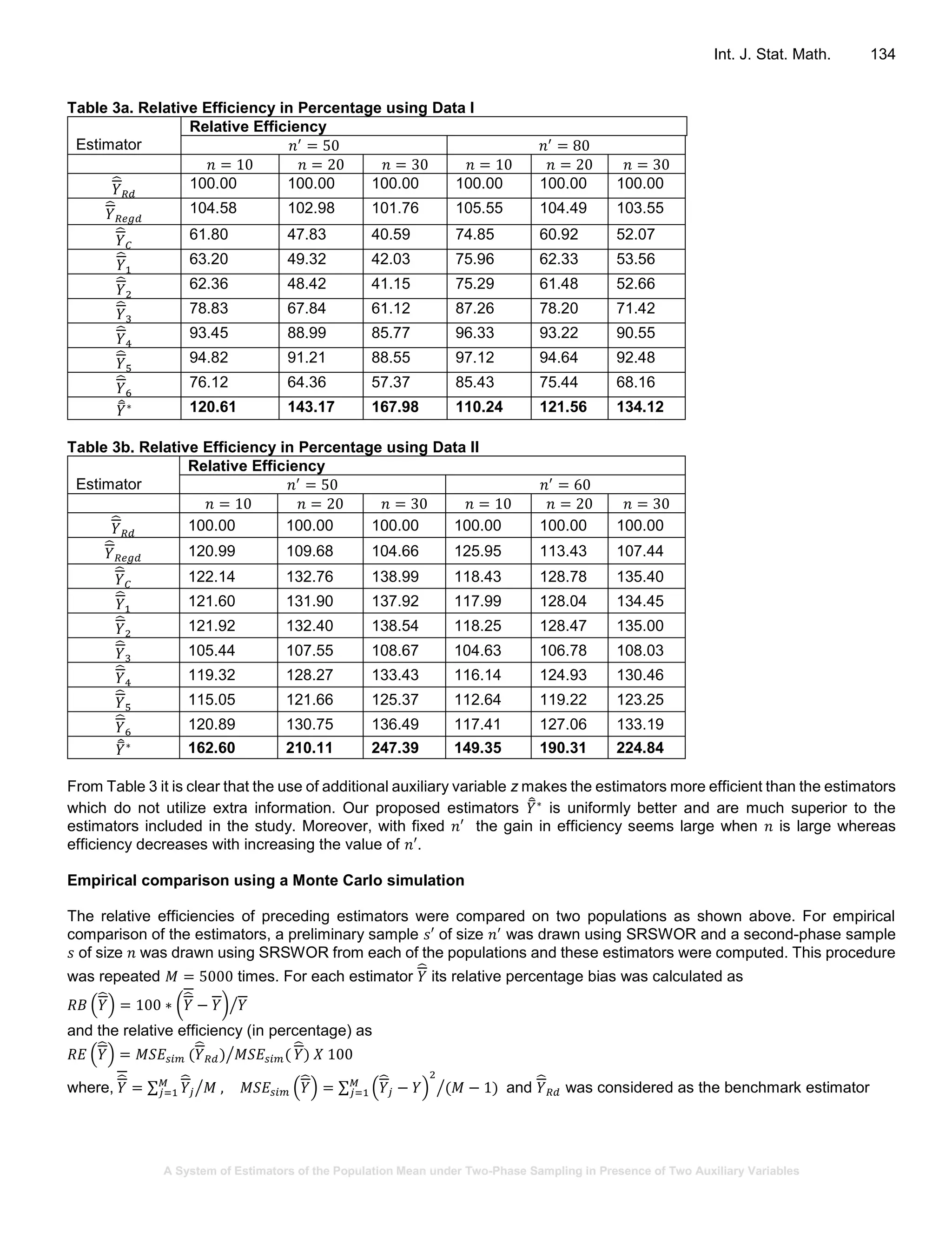
The various estimators discussed in previous sections are now examined using two real data sets.
Data set I : (Jobson, 1992) (The observations are replicated 2 times)
𝑦: Highway Rate
𝑥: Weight
𝑧: Engine size
𝑁 = 194, 𝑛′ = 80, 𝑛 = 30, 𝑌 = 68.37, 𝑋 = 2973.71, 𝑍 = 27.60,
𝜎𝑧 = 12.1268, 𝜌 𝑦𝑥 = 0.7790, 𝜌 𝑦𝑧 = 0.7464, 𝜌 𝑥𝑧 = 0.8862
𝐶 𝑦 = 0.1869, 𝐶 𝑥 = 0.1761, 𝐶𝑧 = 0.4395, 𝛽1(𝑧) = 0.9441, 𝛽2(𝑧) = 2.5386
Data set II : (Fisher, 1936) (The observations are replicated 3 times)
𝑦 = Petal width
𝑥 = Petal length
𝑧 = Sepal length
𝑁 = 150, 𝑛′
= 60, 𝑛 = 30, 𝑌̅ = 1.199, 𝑋̅ = 3.758, 𝑍̅ = 5.483,
𝜎𝑧 = 0.8281, 𝜌 𝑦𝑥 = 0.71, 𝜌 𝑦𝑧 = 0.8179, 𝜌 𝑥𝑧 = 0.8718, 𝐶 𝑦 = 0.6356,
𝐶 𝑥 = 0.4697, 𝐶𝑧 = 0.1417, 𝛽1(𝑧) = 0.3118, 𝛽2(𝑧) = 2.426
To compare performance of the estimators the relative efficiency (in percentage) of an arbitrary estimator 𝑌̂ as compared
to 𝑦̅ is calculated as
𝑅𝐸 (𝑌̂) =
𝑉(𝑦̅)
𝑉(𝑌̂)
× 100%
The REs of various estimators are presented in following tables:

Table 3a. Relative Efficiency in Percentage using Data I
Estimator
Relative Efficiency
𝑛′
= 50 𝑛′
= 80
𝑛 = 10 𝑛 = 20 𝑛 = 30 𝑛 = 10 𝑛 = 20 𝑛 = 30
𝑌̂
𝑅𝑑
100.00 100.00 100.00 100.00 100.00 100.00
𝑌̂
𝑅𝑒𝑔𝑑
104.58 102.98 101.76 105.55 104.49 103.55
𝑌̂
𝐶
61.80 47.83 40.59 74.85 60.92 52.07
𝑌̂
1
63.20 49.32 42.03 75.96 62.33 53.56
𝑌̂
2
62.36 48.42 41.15 75.29 61.48 52.66
𝑌̂
3
78.83 67.84 61.12 87.26 78.20 71.42
𝑌̂
4
93.45 88.99 85.77 96.33 93.22 90.55
𝑌̂
5
94.82 91.21 88.55 97.12 94.64 92.48
𝑌̂
6
76.12 64.36 57.37 85.43 75.44 68.16
𝑌̅̂∗ 120.61 143.17 167.98 110.24 121.56 134.12
Table 3b. Relative Efficiency in Percentage using Data II
Estimator
Relative Efficiency
𝑛′
= 50 𝑛′
= 60
𝑛 = 10 𝑛 = 20 𝑛 = 30 𝑛 = 10 𝑛 = 20 𝑛 = 30
𝑌̂
𝑅𝑑
100.00 100.00 100.00 100.00 100.00 100.00
𝑌̂
𝑅𝑒𝑔𝑑 120.99 109.68 104.66 125.95 113.43 107.44
𝑌̂
𝐶
122.14 132.76 138.99 118.43 128.78 135.40
𝑌̂
1
121.60 131.90 137.92 117.99 128.04 134.45
𝑌̂
2
121.92 132.40 138.54 118.25 128.47 135.00
𝑌̂
3
105.44 107.55 108.67 104.63 106.78 108.03
𝑌̂
4
119.32 128.27 133.43 116.14 124.93 130.46
𝑌̂
5
115.05 121.66 125.37 112.64 119.22 123.25
𝑌̂
6
120.89 130.75 136.49 117.41 127.06 133.19
𝑌̅̂∗ 162.60 210.11 247.39 149.35 190.31 224.84
From Table 3 it is clear that the use of additional auxiliary variable z makes the estimators more efficient than the estimators
which do not utilize extra information. Our proposed estimators 𝑌̅̂∗
is uniformly better and are much superior to the
estimators included in the study. Moreover, with fixed 𝑛′ the gain in efficiency seems large when 𝑛 is large whereas
efficiency decreases with increasing the value of 𝑛′.
Empirical comparison using a Monte Carlo simulation
The relative efficiencies of preceding estimators were compared on two populations as shown above. For empirical
comparison of the estimators, a preliminary sample 𝑠′ of size 𝑛′
was drawn using SRSWOR and a second-phase sample
𝑠 of size 𝑛 was drawn using SRSWOR from each of the populations and these estimators were computed. This procedure
was repeated 𝑀 = 5000 times. For each estimator 𝑌̂ its relative percentage bias was calculated as
𝑅𝐵 (𝑌̂) = 100 ∗ (𝑌̂ − 𝑌) 𝑌⁄
and the relative efficiency (in percentage) as
𝑅𝐸 (𝑌̂) = 𝑀𝑆𝐸𝑠𝑖𝑚 (𝑌̂
𝑅𝑑) 𝑀𝑆𝐸𝑠𝑖𝑚(⁄ 𝑌̂) 𝑋 100
where, 𝑌̂ = ∑ 𝑌̂
𝑗
𝑀
𝑗=1 𝑀 ,⁄ 𝑀𝑆𝐸𝑠𝑖𝑚 (𝑌̂) = ∑ (𝑌̂
𝑗 − 𝑌)
2
𝑀
𝑗=1 (𝑀 − 1)⁄ and 𝑌̂
𝑅𝑑 was considered as the benchmark estimator

Patel and Shah 135
Table 4. Relative Bias and Relative Efficiency in Percentage
Estimator
Relative Bias (%) Efficiency (%)Relative
Population Population
I II I II
𝑛′
= 50,
𝑛 = 20
𝑛′
= 80,
𝑛 = 30
𝑛′
= 50,
𝑛 = 20
𝑛′
= 80,
𝑛 = 30
𝑛′
= 50,
𝑛 = 20
𝑛′
= 80,
𝑛 = 30
𝑛′
= 50,
𝑛 = 20
𝑛′
= 60,
𝑛 = 30
𝑌̂
𝑅𝑑
0.03 -0.03 0.71 0.62 100.00 100.00 100.00 100.00
𝑌̂
𝑅𝑒𝑔𝑑
0.00 -0.03 0.30 0.25 100.32 100.86 108.11 107.06
𝑌̂
𝐶
0.17 0.11 0.61 0.56 46.51 51.39 137.54 136.44
𝑌̂
𝑃𝑑
0.18 -0.03 0.71 0.69 16.92 19.51 73.91 73.87
𝑌̂
1
0.16 0.10 0.60 0.56 47.99 52.88 135.87 135.46
𝑌̂
2
0.17 0.11 0.78 0.56 47.09 51.98 136.18 136.04
𝑌̂
3
0.11 0.07 0.66 0.59 66.29 70.79 108.36 108.25
𝑌̂
4
0.06 0.04 0.62 0.57 87.21 89.98 131.59 131.34
𝑌̂
5
0.06 0.03 0.62 0.57 89.40 91.92 124.82 123.91
𝑌̂
6
0.11 0.07 0.60 0.56 62.85 67.51 134.89 134.16
𝑌̂
7
0.01 0.02 0.33 0.24 83.13 89.43 120.04 119.66
𝑌̂
8
0.06 0.05 0.31 0.21 62.28 69.35 165.87 165.48
𝑌̂
9
-0.00 0.01 0.31 0.21 102.89 107.10 157.87 157.46
𝑌̂
10
0.02 0.02 0.32 0.20 79.58 86.13 164.25 162.27
𝑌̅̂
1
∗ -0.07 -0.05 0.80 0.74 131.47 129.99 226.74 224.86
𝑌̅̂
2
∗ -0.07 -0.06 0.79 0.77 131.44 130.14 220.15 218.29
𝑌̅̂
3
∗ -0.06 -0.05 0.25 0.26 127.45 125.28 119.89 118.24
𝑌̅̂
4
∗ -0.04 -0.04 0.68 0.59 121.33 119.49 254.68 252.16
𝑌̅̂
5
∗ -0.05 -0.05 0.52 0.41 120.72 118.93 219.52 213.56
𝑌̅̂
6
∗ -0.06 -0.05 0.78 0.69 128.43 126.27 242.72 237.67
Table 4 leads to the following comments:
(1) The absolute values of RB’s are all less than 1%.
(2) For large values of 𝐶 𝑥 the estimator 𝑌̅̂
1
∗
and 𝑌̅̂
2
∗
have performed very well compared to the rest of the estimators.
(3) For small values of 𝜎𝑧 the estimator 𝑌̅̂
4
∗
has performed well.
(4) Our proposed estimators (except 𝑌̅̂
3
∗
) have exhibited substantial gain over all the estimators included in the simulation.
CONCLUSION
For many survey populations the relation between survey variable and auxiliary variable is straight line. Also, much often
the extra auxiliary variable that is highly correlated with main auxiliary variable is available. Exploiting these relationships
a system of estimators for the population mean has been suggested, and to compare its performance an empirical study
has been carried out. Theoretically it has been shown that our optimal estimator is most efficient than the estimators
included under the study. Moreover, the suggested estimators have exhibited substantial gain over all the estimators
included in the simulation under certain conditions. These estimators can be further extended in many ways, e.g., using
exponential type estimators in ratio method of estimation, estimation of the population ratio of two study variables, in
presence of non-response etc.
ACKNOWLEDGMENT
The authors are thankful to the editor and anonymous referees for their valuable suggestions which helped to improve the
paper.

REFERENCES
Ahmed, M. S. (2015). Some Improved Estimators in Double Sampling Using two Auxiliary Variables. Sultan Qaboos
University Journal for Science [SQUJS], 19(2), 97-100
Anderson, T. W. (1958). An Introduction to Multivariate Statistical Analysis, Wiley NY.
Bandyopadhyay, A. and Singh, G.N. (2016). Predictive estimation of population mean in two-phase sampling,
Communications in Statistics - Theory and Methods, 45:14, 4249-4267
Chand, L. (1975). Some ratio type estimators based on two or more auxiliary variables, Unpublished Ph. D. thesis, Iowa
State University, Ames, Iowa (USA)
Cochran, W.G. (1977). Sampling Techniques, Wiley, (3rd edition), New York
Dash, P., Mishra, G. (2011). An Improved Class of Estimators in Two-Phase Sampling Using Two Auxiliary Variables.
Communications in Statistics—Theory and Methods. 40. 4347-4352
Fisher, R.A. (1936). The use of multiple measurements in taxonomic problems, Ann. Eugenics 7, 179–188
Jobson, J. D. (1992). Applied Multivariate Data Analysis, Vol. II, Springer-Verlag, New York
Kadilar, C., Cingi, H. (2005). A new ratio estimator using two auxiliary variables. Applied Mathematics and Computation,
162, 901-908
Khan, H. (2016). A Class of Generalized Estimators of Population Mean Using Auxiliary Variables in Single and Two
Phase Sampling with Properties of the Estimators, Unpublished PhD thesis, Department of Statistics, GC University,
Lahore, Pakistan
Khan, H., Khan, M. (2017). New Exponential-Ratio type estimators of Population Mean in Two-Phase Sampling using no
information case on auxiliary variables, Journal of Reliability and Statistical Studies, Vol. 10 (2), 95-103
Khoshnevisan, M., Singh, R., Chauhan, P., Sawan, N., Smarandache, F. (2007). A general family of estimators for
estimating population mean using known value of some population parameter(s). Far east Journal of Theoretical
Statistics, 22, 181-191
Montgomery D.C., Perk E.A., Vining G.G. (2003). Introduction to Linear Regression Analysis, Wiley India Pvt. Ltd. (3rd
Ed.)
Patel, P. A., Shah F. H. (2018). Regression-type Estimators Based on Two Auxiliary Variables of a Finite Population Mean
in Two-phase Sampling, International Journal of Scientific Research in Mathematical and Statistical Sciences, Vol.5,
Issue.5, 144-152
Patel, P. A., Shah F. H. (2018). Two-phase Ratio-type Estimator of a Finite Population Mean, International Journal of
Scientific Research in Mathematical and Statistical Sciences, Vol.5, Issue.5,199-203
Singh H.P., Tailor, R. (2003). Use of known correlation coefficient in estimating the finite population mean. Statistics in
Transition, 6(4), 555-560
Singh, G. N. (2001). On the use of transformed auxiliary variable in estimation of population mean in two-phase sampling,
Statistics in Transition, 5(3), 405-416.
Singh, G.N., Upadhyay, L.N. (1995). A class of modified chain type estimators using two auxiliary variables in two-phase
sampling. Metron LIII, 117-125.
Singh, R., Chauhan, P., Sawan, N., Smarandache, F. (2011). Improvement in estimating population mean using two
auxiliary variables in two-phase sampling, Italian J. of Pure and Applied Mathematics, N-28, 135-142.
Singh, R., Chauhan, P., Sawan, N., Smarandache, F. (2008). Ratio-Product Type Exponential Estimator For Estimating
Finite Population Mean Using Information On Auxiliary Attribute. Pakistan Journal of Statistical Operation Research
4(1) 47-53.
Stuart, A., Ord, K. (1987). Kendall's Advanced Theory of Statistics, Volume 1, Distribution Theory, 4th Edition.
Upadhyay, L. N., Singh, G. N. (2011). Chain type estimators using transformed auxiliary variable in two-phase sampling,
Advances in Modeling and Analysis, 38 (1-2), 1-10.
Upadhyaya, L.N., Singh, H.P. (1999). Use of transformed auxiliary variable in estimating the finite population mean.
Biometrical Journal, 41, 5, 627-636.
Vishwakarma, G. K., Kumar, M. (2014). “An Improved Class of Chain Ratio-Product Type Estimators in Two-Phase
Sampling Using Two Auxiliary Variables,” Journal of Probability and Statistics, Article ID 939701.
Accepted 16 May 2019
Citation: Patel PA, Shah FH (2019). A System of Estimators of the Population Mean under Two-Phase Sampling in
Presence of Two Auxiliary Variables. International Journal of Statistics and Mathematics, 6(2): 130-136.
Copyright: © 2019 Patel and Shah. This is an open-access article distributed under the terms of the Creative Commons
Attribution License, which permits unrestricted use, distribution, and reproduction in any medium, provided the original
author and source are cited.

A System of Estimators of the Population Mean under Two-Phase Sampling in Presence of Two Auxiliary Variables

More Related Content

What's hot

Similar to A System of Estimators of the Population Mean under Two-Phase Sampling in Presence of Two Auxiliary Variables

More from Premier Publishers

Recently uploaded

A System of Estimators of the Population Mean under Two-Phase Sampling in Presence of Two Auxiliary Variables