Class of Estimators of Population Median Using New Parametric Relationship for Median

International Journal of Mathematics and Statistics Invention (IJMSI)
E-ISSN: 2321 – 4767 P-ISSN: 2321 - 4759
www.ijmsi.org Volume 5 Issue 2 || February. 2017 || PP-41-48
www.ijmsi.org 41 | Page
Class of Estimators of Population Median Using New Parametric
Relationship for Median
M.K. Sharma1
, Sarbjit S. Brar2
and Harinder Kaur3*
1
(Department of Statistics, Punjabi University, Patiala, Punjab, India.)
2
3
ABSTRACT: In this paper, we have defined a class of estimators of population median using the known
information of population mean (𝑋) of the auxiliary variable making use of new parametric relationship for
population median. We have derived the asymptotic expression for the MSE of any estimator of the proposed
class and also its minimum value. As minimum MSE of all the estimators of defined class are same so to choose
the optimum estimator of the class for the given population w.r.t.bias also, we have considered some important
sub-classes of the generalized class. The optimum biases of the considered estimators are obtained (up to terms
of order 𝑛−1) and compared with each other. Theoretical results are supported by an empirical study based on
twelve populations to show the superiority of the suggested estimator over others.
KEYWORDS:Auxiliary variable, SRSWOR, Bias, Mean square error, Median, Mode, Coefficient of skewness.
I. INTRODUCTION
In many situations, population median is regarded as a more appropriate measure of central tedency than
arithmetic mean such as when we are interested in the positional average as a measure of central tendency which
is not affected much by extreme observations i.e. for skewed distributions or we are dealing with attributes or
qualitative characters which can not be measured quantitatively but still can be arranged in ascending or
decending order of magnitude. When it is unknown then in above situations, one is interested to estimate it.
Initially, estimation of population median without auxiliary variable was materialized, after that some authors
including Kuk and Mak (1989), Mak and Kuk(1993) , Garcia and Cebrian (2001), Singh et al. (2006), Al and
Cingi (2010), Singh and Solanki (2013) used the known auxiliary information in estimation of population
median.
Recently, Sharma et al (2016b) established the new parametric relationship for population median (𝑀𝑑) as
𝑀𝑑 = 𝑌 −
𝑘1
3
𝜇30
𝑆𝑦
2
where for the 𝑌- population 𝑘1 =
𝛽 𝑦
𝜆 𝑦
is known constant. They proposed mean per unit estimator, the ratio-type
and product-type estimators of population median 𝑀𝑑 under the different situations as
𝑀𝑑1
′
= 𝑦 −
𝑘1𝑜𝑝𝑡
3
𝑚30
𝑠𝑦
2
,
𝑀𝑑2
′
= 𝑦
𝑋
𝑥
−
𝑘2𝑜𝑝𝑡
3
𝑚30
𝑠𝑦
2
𝑋
𝑥
,
and 𝑀𝑑3
′
= 𝑦
𝑥
𝑋
−
𝑘3𝑜𝑝𝑡
3
𝑚30
𝑠𝑦
2
𝑥
𝑋
where 𝑘1𝑜𝑝𝑡 =
𝛽 𝑦
𝜆 𝑦
, 𝑘2𝑜𝑝𝑡 =
𝛽 𝑦 𝐶 𝑦 +𝛽1𝑦 𝐶 𝑥
2−𝐶 𝑦𝑥 +𝐵
𝐶 𝑦 𝜆 𝑦 +𝛽1𝑦
2 𝐶 𝑥
2−2𝛽1𝑦 𝐵
and 𝑘3𝑜𝑝𝑡 =
𝛽 𝑦 𝐶 𝑦 +𝛽1𝑦 𝐶 𝑥
2+𝐶 𝑦𝑥 −𝐵
𝐶 𝑦 𝜆 𝑦 +𝛽1𝑦
2 𝐶 𝑥
2+2𝛽1𝑦 𝐵
are the conventional
consistent estimators of the constants 𝑘1, 𝑘2 and 𝑘3. Here the estimator 𝑀𝑑1
′
uses no information on auxiliary
variable 𝑥 which is highly correlated with 𝑦, whereas 𝑀𝑑2
′
and 𝑀𝑑3
′
uses the known information of 𝑋, which are
of ratio-type and product-type estimators respectively.
In the present paper, we propose a class of estimators of population median using the new parametric
relationship for population median when the population mean (𝑋) of the auxiliary variable is known.
Asymptotic expressions for the Bias and MSE of any estimator of the proposed class and also its minimum
value are obtained. We also consider some important members of the proposed class and up to the first degree of
approximation the minimum MSE’s of the considered estimators are same but biases are different. To have the
rough idea about the optimum biases of the considered estimators and minmimum MSE of estimators of the
class numerical illustration is given.

Class of Estimators of Population Median Using New Parametric Relationship for Median
II. NOTATIONS AND EXPECTATIONS
Suppose a simple random sample of size 𝑛 is drawn from a finite population of size 𝑁 without replacement and observations
on both study variables 𝑦 and auxiliary variable 𝑥 are taken. Let the values of variable 𝑦 and 𝑥 be denoted by 𝑌𝑖 and 𝑋𝑖
respectively on the 𝑖 𝑡ℎ unit of the population 𝑖 = 1,2 … 𝑁 and the corresponding small letters 𝑦𝑖 and 𝑥𝑖 denote the sample
values.
Taking,
𝑌 =
1
𝑁
𝑌𝑖
𝑁
𝑖=1
, 𝑋 =
1
𝑁
𝑋𝑖
𝑁
𝑖=1
𝑆 𝑦
2
=
1
𝑁 − 1
𝑌𝑖 − 𝑌 2
𝑁
𝑖=1
, 𝑆 𝑥
2
=
1
𝑁 − 1
𝑋𝑖 − 𝑋 2
𝑁
𝑖=1
𝜇 𝑟𝑠 =
1
𝑁
𝑌𝑖 − 𝑌 𝑟
𝑁
𝑖=1
𝑋𝑖 − 𝑋 𝑠
, 𝜆 𝑟𝑠 =
𝜇 𝑟𝑠
𝜇20
𝑟 2
𝜇02
𝑠 2
𝑚30 =
𝑛
𝑛 − 1 𝑛 − 2
𝑦𝑖 − 𝑦 3
𝑛
𝑖=1
,
Obviously
𝜆11 = 𝜌𝑥𝑦 = 𝜌(Correlation between 𝑥 and 𝑦)
𝜆30 = 𝛽1𝑦 (Coefficient of skewness of 𝑦)
𝜆40 = 𝛽2𝑦 (Coefficient of kurtosis of 𝑦)
Defining,
𝛿0 =
𝑦
𝑌
− 1, 𝛿 =
𝑠 𝑦
2
𝑆 𝑦
2 − 1
𝜖 =
𝑥
𝑋
− 1, 𝜂1 =
𝑚30
𝜇30
− 1
For the sake of simplicity, assume that 𝑁 is large enough as compares to 𝑛 so that finite population correction (fpc) terms are
ignored throughout.
For the given SRSWOR, we have the following expectations,
𝐸 𝛿0 = 𝐸 𝛿 = 𝐸 𝜖 = 0 𝐸 𝛿0
2
=
1
𝑛
𝐶 𝑦
2
𝐸 𝜖2
=
1
𝑛
𝐶𝑥
2
, 𝐸 𝛿0 𝜖 =
1
𝑛
𝐶 𝑦𝑥
𝐸 𝜖𝛿 =
1
𝑛
𝜆21 𝐶𝑥 𝐸 𝛿0 𝛿 =
1
𝑛
𝜆30 𝐶 𝑦 =
1
𝑛
𝛽1𝑦 𝐶 𝑦
and up to terms of order 𝑛−1
𝐸 𝜂1 = 0
𝐸 𝛿2
=
1
𝑛
𝜆40 − 1 =
1
𝑛
𝛽2𝑦 − 1 ,
𝐸 𝜂1
2
=
1
𝑛
𝜆60 − 6𝜆40 − 𝜆30
2
+ 9
𝜆30
2 =
1
𝑛
𝜆60 − 6𝛽2𝑦 − 𝛽1𝑦
2
+ 9
𝛽1𝑦
2 ,
𝐸 𝛿0 𝜂1 =
1
𝑛
𝜆40 − 3
𝜆30
𝐶 𝑦 =
1
𝑛
𝛽2𝑦 − 3
𝛽1𝑦
𝐶 𝑦,
𝐸 𝛿𝜂1 =
1
𝑛
𝜆50 − 4𝜆30
𝜆30
=
1
𝑛
𝜆50 − 4𝛽1𝑦
𝛽1𝑦
,
𝐸 𝜖𝜂1 =
1
𝑛
𝜆31 − 3𝜌
𝜆30
𝐶𝑥 =
1
𝑛
𝜆31 − 3𝜌
𝛽1𝑦
𝐶𝑥.
III. PROPOSED CLASS OF ESTIMATORS
Sharma et al. (2016a) defined the class of estimators of population mode 𝑀𝑜 as
𝑀𝑜𝑔 = 𝑀𝑜 𝑡(𝑢) (3.1)
where the optimum values of two unknown constants 𝑘 and 𝑡(1) were determined by minimizing the MSE’s up to terms of
order 𝑛−1
, the minimum MSE was obtained as
𝑀𝑆𝐸 𝑚𝑖𝑛 =
1
𝑛
𝑌2
𝐶 𝑦
2
1 − 𝜌2
−
(𝐵𝑦 𝜌 + 𝛽𝑦 )2
(𝜆 𝑦 − 𝐵𝑦
2
)
(3.2)
where
𝜆 𝑦 = 𝜆60 − 6𝛽𝑦 + 𝛽0𝑦
𝛽𝑦 = 𝛽2𝑦 − 𝛽1𝑦
2
− 3,
𝛽0𝑦 = 𝛽1𝑦
2
𝛽2𝑦 − 2𝛽1𝑦 𝜆50 − 9,
𝐵𝑦 = 𝛽1𝑦 𝜆21 − 𝜆31 + 3𝜌

If we define the wider class of estimators of population mode 𝑀𝑜 as
𝑀𝑜𝑔 = 𝑡(𝑀𝑜, 𝑢) (3.3)
Two constants 𝑘 and 𝑡1 are involved in the class (3.3) and their optimum values determined by minimizing the MSE, up to
terms of order 𝑛−1
, are
𝑘 =
𝐵𝑦 𝜌 + 𝛽𝑦
𝜆 𝑦 − 𝐵𝑦
2
(3.4)
𝑡1 = −
𝑌 𝐶 𝑦 𝐵𝑦 𝛽𝑦 + 𝜌𝜆 𝑦
𝐶𝑥 𝜆 𝑦 − 𝐵𝑦
2
Up to terms of order 𝑛−1, the minimum MSE of the optimum estimator of class (3.3) is same as the minimum MSE of the
optimum estimator of class (3.1) defined by Sharma et al. (2016a).
We, here propose a generalized class of estimators of population median (𝑀 𝑑 ) when 𝑋 is known,
𝑀 𝑑𝑔 = ℎ(𝑀 𝑑 , 𝑢) (3.5)
where 𝑀 𝑑 = 𝑦 −
𝑘
3
𝑚30
𝑠 𝑦
2 and 𝑘 is constant whose value is given by (3.4). Whatever be the sample chosen, let 𝑢 =
𝑥
𝑋
assume
values in a bounded closed convex subset 𝑅 of the two-dimensional real space. Let ℎ(𝑀 𝑑, 𝑢) be a function of 𝑀 𝑑 and 𝑢 such
that
ℎ 𝑀 𝑑, 1 = 𝑀 𝑑
and such that it satisfies the following conditions:
(i) The function ℎ(𝑀 𝑑 , 𝑢) is continuous and bounded in 𝑅.
(ii) The first and second order partial derivatives of ℎ(𝑀 𝑑 , 𝑢) exist and are continuous and bounded in 𝑅.
⇒ ℎ1 𝑀 𝑑 , 1 = 1
where ℎ1 𝑀 𝑑 , 1 is the first order partial derivative of function ℎ(𝑀 𝑑 , 𝑢).
Note that the estimators of population median 𝑀 𝑑 defined by Sharma et al. (2016) are the members of the proposed class
of estimators (3.5).
To find the biases and 𝑀𝑆𝐸′𝑠 of estimators of class 𝑀 𝑑𝑔 , we expand the function ℎ(𝑀 𝑑, 𝑢) about the value (𝑀 𝑑 , 1) in
second-order Taylor’s series, writing it in terms of 𝛿0, 𝛿, 𝜖, 𝜂1and then taking the expectations given in section 2, up to
terms of order𝑛−1, we get,
𝐵𝑖𝑎𝑠 𝑀 𝑑𝑔 = 𝑂(𝑛−1) (3.6)
𝑀𝑆𝐸 𝑀 𝑑𝑔 =
1
𝑛
𝑌2 𝐶 𝑦
2 + ℎ1
2
𝐶𝑥
2 + 2ℎ1 𝑌 𝐶 𝑦𝑥 +
𝑘2
9
𝑌2 𝐶 𝑦
2 𝜆 𝑦 −
2
3
𝑘𝑌2 𝐶 𝑦
2 𝛽𝑦 +
2
3
ℎ1 𝑘𝑌 𝐶 𝑦 𝐶𝑥 𝐵𝑦 (3.7)
as 𝑘 is known constant, whose value is given by (3.4) above, so the only unknown constant here to find out is ℎ1 =
𝜕ℎ𝜕𝑢𝑢=1 whose value is determined by minimizing 𝑀𝑆𝐸(𝑀𝑑𝑔).
To obtain the minimum value of 𝑀𝑆𝐸(𝑀 𝑑𝑔 ) we differentiate (3.7) w.r.t. ℎ1, then equating to zero, we get,
ℎ1 𝐶𝑥 + 𝑌 𝜌𝐶 𝑦 +
𝑘
3
𝑌 𝐶 𝑦 𝐵𝑦 = 0
Solving above equation by substitute the value of 𝑘 𝑜𝑝𝑡 for ℎ1, we get
ℎ1 = −
𝑌 𝐶 𝑦 {3𝜌𝜆 𝑦 − 2𝜌𝐵𝑦
2
+ 𝛽𝑦 𝐵𝑦 }
3𝐶𝑥{𝜆 𝑦 −𝐵𝑦
2
}
Substituting the values of pair (𝑘1, 𝑡 1 ) in (3.7), we get,
𝑀𝑆𝐸 𝑚𝑖𝑛 𝑀𝑑𝑔 =
1
𝑛
𝑌2
𝐶 𝑦
2
{1 − 𝜌2
−
5(𝐵𝑦 𝜌 + 𝛽𝑦 )2
9{𝜆 𝑦 − 𝐵𝑦
2
}
}
From Srivastava and Jhajj (1983) results, here we can also say that the unknown population parameters in optimum values of
constants will not create any problem for practical use of the proposed class 𝑀 𝑑𝑔 . We can construct the large number of
estimators belonging to the proposed class 𝑀 𝑑𝑔 . Here it should be noted that the use of estimators of the proposed class
𝑀 𝑑𝑔 require the optimum values of constants 𝑘 andℎ1 , which are further functions of unknown population parameter.
However, if it is possible to guess accurately the values of such parameters either through past experience or through a pilot
sample survey, then the values of optimum constants so obtained by using these guessed values of parameters are close
enough to the optimum values of constants and the resulting estimators will be better than the convention estimators. Even if
we replace the parameters in the constants 𝑘 and ℎ1 by their conventional consistent estimators then up to terms of order
𝑛−1, the minimum 𝑀𝑆𝐸 𝑀 𝑑𝑔 remains the same.
Remarks:
(i.) Up to terms of order 𝑛−1
,
𝑀𝑆𝐸 𝑚𝑖𝑛 𝑀 𝑑𝑔 < 𝑀𝑆𝐸 𝑌𝑙𝑟
iff

5 𝐵𝑦 𝜌 + 𝛽𝑦
2
9 𝜆 𝑦 − 𝐵𝑦
2
> 0
(ii.) Special Case of Bivariate Normal Population
Let (𝑌, 𝑋)~𝑁(𝜇 𝑦 , 𝜇 𝑥 , 𝜎𝑦
2
, 𝜎𝑥
2
, 𝜌), then we have 𝜆60 = 15, 𝜆40 = 3, 𝜆31 = 3𝜌, 𝜆22 = 1 + 2𝜌2
,𝜆 𝑟,𝑠 = 0 if 𝑟 + 𝑠 is odd. Also,
𝑋~𝑁(𝜇 𝑥, 𝜎𝑥
2
) and 𝑌~𝑁(𝜇 𝑦 , 𝜎𝑦
2
).
Using these values, we get,
𝑀𝑆𝐸 𝑚𝑖𝑛 𝑀 𝑑𝑔 = 𝑀𝑆𝐸 𝑌𝑙𝑟 =
1
𝑛
𝑆 𝑦
2
(1 − 𝜌2
)
IV. SOME IMPORTANT MEMBERS OF THE PROPOSED CLASS
Any estimator, which satisfies the stated regularities conditions of the proposed class of estimators (3.5), is a member of the
class. So we can construct a large number of estimators of 𝑀 𝑑 . All the estimators of the class though have the same
minimum MSE (up to terms of order 𝑛−1) but their biases are different. To choose the optimum estimator of the proposed
class, we have to choose that estimator which has the minimum MSE as well as the minimum bias. Hence to choose the
optimum estimator of the class, we take into consideration the following important sub-classes of the proposed generalized
class (3.5) as
𝑀 𝑑𝑔
(1)
= 𝑀 𝑑 + 𝛼1 𝑢 − 1 (4.1)
𝑀 𝑑𝑔
(2)
= 𝑀 𝑑 exp 𝛼2 𝑙𝑜𝑔𝑢 (4.2)
𝑀 𝑑𝑔
(3)
= 𝑀 𝑑 {1 + 𝛼3 𝑢 − 1 } (4.3)
and 𝑀 𝑑𝑔
(4)
= 𝑀 𝑑 exp⁡{𝛼4 𝑢 − 1 } (4.4)
Expanding above four estimators in a second order Taylor’s series and using the expectations given in section II, we obtain,
𝐵𝑖𝑎𝑠 𝑀 𝑑𝑔
1
=
1
𝑛
𝑘
3
𝑌 𝐶 𝑦 𝜆50 − 𝛽1𝑦 𝛽2𝑦 + 3
2
=
1
𝑛
𝑘
3
𝑌 𝐶 𝑦 𝜆50 − 𝛽1𝑦 𝛽2𝑦 + 3 + 𝛼2 𝑌 𝐶 𝑦𝑥 +
𝑘
3
𝛼2 𝑌 𝐶 𝑦 𝐶𝑥 𝐵𝑦 −
1
2
𝛼2 𝑀 𝑑 𝐶𝑥
2
+
1
2
𝛼2
2
𝑀 𝑑 𝐶𝑥
2
3
=
1
𝑛
𝑘
3
𝑌 𝐶 𝑦 𝜆50 − 𝛽1𝑦 𝛽2𝑦 + 3 + 𝛼3 𝑌 𝜌𝐶𝑥 +
𝑘
3
𝛼3 𝑌 𝐶𝑥 𝐵𝑦
4
=
1
𝑛
𝑘
3
𝑌 𝐶 𝑦 𝜆50 − 𝛽1𝑦 𝛽2𝑦 + 3 + 𝛼4 𝑌 𝐶 𝑦𝑥 +
𝑘
3
𝛼4 𝑌 𝐶 𝑦 𝐶𝑥 𝐵𝑦 +
1
2
𝛼4
2
𝑀 𝑑 𝐶𝑥
2
and
𝑀𝑆𝐸 𝑀 𝑑𝑔
1
=
1
𝑛
𝑌2
𝐶 𝑦
2
+ 𝛼1
2
𝐶𝑥
2
+ 2𝛼1 𝑌 𝐶 𝑦𝑥 +
𝑘2
9
𝑌2
𝐶 𝑦
2
𝜆 𝑦 −
2
3
𝑘𝑌2
𝐶 𝑦
2
𝛽𝑦 +
2
3
𝑘𝛼1 𝑌 𝐶 𝑦 𝐶𝑥 𝐵𝑦
𝑀𝑆𝐸 𝑀 𝑑𝑔
𝑖
=
1
𝑛
𝑌2
𝐶 𝑦
2
+ 𝛼𝑖
2
𝑀 𝑑
2
𝐶𝑥
2
+ 2𝛼𝑖 𝑀 𝑑 𝑌 𝐶 𝑦𝑥 +
𝑘2
9
𝑌2
𝐶 𝑦
2
𝜆 𝑦 −
2
3
𝑘𝑌2
𝐶 𝑦
2
𝛽𝑦
+
2
3
𝑘𝛼𝑖 𝑀 𝑑 𝑌 𝐶𝑦 𝐶𝑥 𝐵𝑦 ; 𝑖 = 2,3,4.
where𝑘 is known constant, whose value is given by (3.4) above and the only unknown constant here to find out is 𝛼𝑖 ,
𝑖 = 1,2,3,4, whose value is determined by minimizing the respective 𝑀𝑆𝐸(𝑀 𝑑𝑔
𝑖
). Then the MSE of 𝑀 𝑑𝑔
𝑖
, 𝑖 = 1,2,3,4 are
minimised for
𝛼1 = −
𝑌 𝐶 𝑦 3𝜌𝜆 𝑦 − 2𝜌𝐵𝑦
2
+ 𝛽𝑦 𝐵𝑦
3𝐶𝑥 𝜆 𝑦 −𝐵𝑦
2
,
And
𝛼𝑖 = −
2
+ 𝛽𝑦 𝐵𝑦
3𝑀 𝑑 𝐶𝑥 𝜆 𝑦−𝐵𝑦
2
; 𝑖 = 2,3,4.
and the optimum biases and minimum MSE are given as,
𝐵𝑖𝑎𝑠 𝑜𝑝𝑡 (𝑀 𝑑𝑔
(1)
) =
1
𝑛
𝐵𝑦 𝜌 + 𝛽𝑦
3(𝜆 𝑦−𝐵𝑦
2
)
𝑌 𝐶 𝑦 𝜆50 − 𝛽1𝑦 𝛽2𝑦 + 3
(2)
) =
1
𝑛
𝑌 𝐶 𝑦
2
)
𝐵𝑦 𝜌 + 𝛽𝑦 𝜆50 − 𝛽1𝑦 𝛽2𝑦 + 3
−
2
+ 𝛽𝑦 𝐵𝑦
2
6𝑀 𝑑(𝜆 𝑦−𝐵𝑦
2
)
+
𝐶𝑥
2
3𝜌𝜆 𝑦 − 2𝜌𝐵𝑦
2 + 𝛽𝑦 𝐵𝑦

(3)
) =
1
𝑛
𝑌 𝐶 𝑦
2)
𝐵𝑦 𝜌 + 𝛽𝑦 𝜆50 − 𝛽1𝑦 𝛽2𝑦 + 3
−
2
+ 𝛽𝑦 𝐵𝑦
2
2)
(4)
) =
1
𝑛
𝑌 𝐶 𝑦
2)
𝐵𝑦 𝜌 + 𝛽𝑦 𝜆50 − 𝛽1𝑦 𝛽2𝑦 + 3
−
2
+ 𝛽𝑦 𝐵𝑦
2
2
)
and
𝑀𝑆𝐸 𝑚𝑖𝑛 𝑀 𝑑𝑔
𝑖
=
1
𝑛
𝑌2
𝐶 𝑦
2
1 − 𝜌2
−
5 𝐵𝑦 𝜌 + 𝛽𝑦
2
2
; 𝑖 = 1,2,3,4.
V. COMPARISION W.R.T. BIASES
Theorem 1. Up to terms of order 𝑛−1
,
𝐵𝑖𝑎𝑠 𝑜𝑝𝑡 𝑀 𝑑𝑔
(1)
< 𝐵𝑖𝑎𝑠 𝑜𝑝𝑡 𝑀 𝑑𝑔
(2)
iff
(1) 2
(2) 2
when
𝐺 >
6𝐶𝑥 𝜆 𝑦 − 𝐵𝑦
2
𝐿1
2 2𝐿2 +
𝐶𝑥 𝐿1
2
𝑜𝑟 𝐺 <
3𝐶𝑥 𝜆 𝑦 − 𝐵𝑦
2
𝐿1
where 𝐿1 = 3𝜌𝜆 𝑦 − 2𝜌𝐵𝑦
2
+ 𝛽𝑦 𝐵𝑦 , 𝐿2 = 𝐵𝑦 𝜌 + 𝛽𝑦 𝜆50 − 𝛽1𝑦 𝛽2𝑦 + 3 and 𝐺 =
𝑌 𝐶 𝑦
𝑀 𝑑
.
,
(1)
(3)
iff
(1) 2
(3) 2
when
𝐺 >
6𝐿2 𝜆 𝑦 − 𝐵𝑦
2
𝐿1
2 .
,
(1)
(4)
iff
(1) 2
(4) 2
when
𝐺 >
12𝐿2 𝜆 𝑦 − 𝐵𝑦
2
𝐿1
2 .
,
(2)
(3)
iff
(2) 2
(3) 2
when
𝐺 >
2
𝐿1
2 𝐿2 −
𝐶𝑥 𝐿1
2
+ 𝐿2
2
−
𝐶𝑥
2
𝐿1
2
2
− 4𝐶𝑥 𝐿1 𝐿2
𝑜𝑟 𝐺 <
2
𝐿1
2 𝐿2 −
𝐶𝑥 𝐿1
2
− 𝐿2
2
−
𝐶𝑥
2 𝐿1
2
2
− 4𝐶𝑥 𝐿1 𝐿2 .
,
(2)
(4)
iff

(2) 2
(4) 2
when
𝐺 >
2
𝐿1
2
𝐶𝑥 𝐿1
4
+ 𝐿2 .
Theorem 6. Up to terms of order 𝑛−1,
(3)
(4)
iff
(3) 2
(4) 2
when
𝐺 <
4𝐿2 𝜆 𝑦 − 𝐵𝑦
2
𝐿1
2 .
VI. NUMERICAL ILLUSTRATIONS
To illustrate the result numerically, we have made computations for 12 populations taken from literature by using Microsoft
Excel 2010.
The source of the populations, the nature of the variables, the values of 𝑌, 𝑘1,𝜇20, 𝛽1𝑦 and 𝜌 are listed in Table 1.
The efficiencies of proposed estimators are given in Table 2.
The absolute optimum biases of considered four important sub-classes of the proposed generalized class are given in Table
3. In Table 4, we compare optimum estimator of proposed class with all 22 existing estimators of different technique that are
listed by Singh and Solanki (2013), 3 existing estimators defined by Sharma et al. (2016b) and the linear regression estimator
of meadian 𝑀 𝑑.
Table 1: Description of populations
Sr.
No.
Source
𝒚 𝒙 𝒀 𝒌 𝟏 𝝁 𝟐𝟎 𝜷 𝟏𝒚 𝝆
1 Murthy (1967),
p.91 (1-35)
Cultivated
area (acres)
Holding size
(acres)
2.3650 -0.2217 1.5818 0.9119 0.3685
2 Murthy (1967),
p.398
No. of
absentees
No. of
workers
9.6512 0.0442 42.1341 1.5575 0.6608
3 Murthy (1967),
p.399
Area under
wheat in
1964
Cultivated
area in 1961 199.4412 -0.0220
21900.893
6
1.1295 0.9043
4 Chakravarty et
al.(1967),
p-183
Length(cm)
measured by
1st
person
Length(cm)
measured by
2nd
person
4.9737 -0.0437 0.1346 -0.0546 0.9317
5 Chakravarty et
al.(1967),
p-207
Weight
(kg) of male
Height
(cm) of male 29.2625 -0.0240 6.5836 0.3670 0.7709
6 Chakravarty et
al.(1967),
p-207
Weight (kg)
of female
Height (cm)
of female 28.5313 -0.3896 1.8109 0.1099 0.2306
7 Chakravarty et
al.(1967),
p-185 (1-35)
Weight (lb)
of Kayastha
males
Stature (cm)
of Kayastha
males
82.2000 -0.2012 191.7029 0.0439 0.8578
8 Chakravarty et
al.(1967),
p-185 (1-76)
Weight (lb)
of Kayastha
males
Stature (cm)
of Kayastha
males
89.4211 0.0516 278.4806 0.6068 0.4361
9 Chochran
(1999), p-325
Total
number of
persons
Average
persons per
room
101.1000 -0.3015 214.6900 0.3248 0.6515
10 Maddala&Lahi
ri (1992),
p-316
Consumptio
n per capital
of Lamb
Deflated
prices of
Lamb
4.5188 -0.0281 0.2103 -0.6578 -0.7517
11 Guajrati
(2004),
p-27,(1-50)
Price per
dozen(cent)
in 1990
Egg
production
in 1991
(million)
78.2880 0.0111 445.3787 0.9959 -0.3096
12 http://content.h
ccfl.edu
Highway
fuel
efficiency of
vehicles (in
miles)
Weightof
vehicles (in
1000 lbs.) 30.6154 -0.2045 15.6213 0.0549 -0.8978

Table 2: 𝒏−𝟏
× 𝑴𝑺𝑬′𝒔 of 𝑴 𝒅 𝟏
, 𝑴 𝒅 𝟐
, 𝑴 𝒅 𝟑
, 𝒀 𝑹,𝒀 𝑷, 𝑴 𝒅𝒈 and 𝑴𝒍𝒓 up to terms of order 𝒏−𝟏
𝒏−𝟏 ∗ 𝑴𝑺𝑬′𝒔 of
Pop. No. 𝑴 𝒅 𝟏
𝑴 𝒅 𝟐
𝑴 𝒅 𝟑 𝒀 𝑹 𝒀 𝑷
𝑴 𝒅𝒈 𝑴𝒍𝒓
1 1.4201 7.2895 14.9915 - - 1.2843 1.3670
2 40.3890 22.9990 90.9751 23.7459 - 22.9937 23.7380
3 20935.5069 4172.6821 66661.3002 4286.448
3
- 3971.8559 3992.7274
4 0.1201 0.0201 0.4947 0.0201 - 0.0175 0.0178
5 6.5145 3.9238 10.5213 3.9590 - 2.6658 2.6713
6 1.5012 1.8675 2.6333 - - 1.4462 1.7146
7 142.0275 79.4387 237.1650 105.5227 - 45.2976 50.6533
8 270.2905 228.2034 539.9383 237.2253 - 216.9131 225.5076
9 176.6954 125.6235 554.3948 135.1725 - 106.0736 123.5609
10 0.2005 0.6691 0.1023 - 0.1023 0.0912 0.0915
11 445.3506 10052.185
1
7317.9041 - - 402.4026 402.7018
12 10.6760 59.4203 6.4059 - 6.7647 2.7241 3.0308
Table 3: 𝒏−𝟏
× 𝑩𝒊𝒂𝒔 𝒐𝒑𝒕 of 𝑴 𝒅𝒈
(𝒊)
, 𝒊 = 𝟏, 𝟐, 𝟑, 𝟒, up to terms of order 𝒏−𝟏
Pop. No. 𝑩𝒊𝒂𝒔 𝒐𝒑𝒕(𝑴 𝟏𝒅) 𝑩𝒊𝒂𝒔 𝒐𝒑𝒕(𝑴 𝟐𝒅) 𝑩𝒊𝒂𝒔 𝒐𝒑𝒕(𝑴 𝟑𝒅) 𝑩𝒊𝒂𝒔 𝒐𝒑𝒕(𝑴 𝟒𝒅)
1 0.0355 0.2832 0.0485 0.0065
2 0.7019 0.5424 1.5368 0.4174
3 1.0521 24.3762 125.6609 63.3565
4 0.0008 0.0025 0.0223 0.0107
5 0.0042 0.0425 0.1376 0.0709
6 0.0383 0.0355 0.0406 0.0395
7 0.0131 0.4398 1.4981 0.7425
8 1.8005 1.9346 1.1957 1.4981
9 0.4794 0.3064 1.2792 0.8793
10 0.0044 0.0253 0.0210 0.0083
11 0.2729 3.9549 0.2967 0.0119
12 0.0172 0.4966 0.3830 0.2001
Table 4: MSE and Relative Efficiencies of Population Median Class
MSE Relative Efficiency
Estimators Pop.I Pop.II Pop.I Pop.II
𝑉(𝑀 𝑦) 565443.57 565443.57 100.00 100.00
𝑀𝑆𝐸(𝑀𝑟) 988372.76 536149.50 57.21 105.46
𝑀𝑆𝐸 𝑚𝑖𝑛 (𝑀 𝑑)
𝑀𝑆𝐸 𝑚𝑖𝑛 (𝑀 𝑦
(𝐺)
) 552636.13 508766.02 102.32 111.14
𝑀𝑆𝐸 𝑚𝑖𝑛 (𝑀𝑖)
𝑀𝑆𝐸 𝑚𝑖𝑛 (𝑡4) 630993.68 478781.74 89.61 118.10
𝑀𝑆𝐸 𝑚𝑖𝑛 (𝑡5) 499412.60 499412.60 113.22 113.22
𝑀𝑆𝐸 𝑚𝑖𝑛 (𝑡6) 630979.49 478784.18 89.61 118.10
𝑀𝑆𝐸 𝑚𝑖𝑛 (𝑡7) 630367.71 478806.00 89.70 118.09
𝑀𝑆𝐸 𝑚𝑖𝑛 (𝑡8) 522345.11 488388.99 108.25 115.78
𝑀𝑆𝐸 𝑚𝑖𝑛 (𝑡9) 630993.63 478781.75 89.61 118.10
𝑀𝑆𝐸 𝑚𝑖𝑛 (𝑡10) 489754.69 493940.28 115.45 114.48
𝑀𝑆𝐸 𝑚𝑖𝑛 (𝑡11) 630993.67 478781.74 89.61 118.10
𝑀𝑆𝐸 𝑚𝑖𝑛 {𝑀 𝑑
(1)
} 489569.06 495484.97 115.50 114.12
(2)
} 489395.24 454675.78 115.54 124.36
(3)
} 3220.01 51355.17 17560.30 1101.05
𝑀𝑆𝐸 𝑚𝑖𝑛 {𝑀 𝑑1
(4)
} 480458.29 454616.16 117.69 124.38
(4)
} 489395.24 454675.78 115.54 124.36
(4)
} 480459.82 454616.17 117.69 124.38
(4)
} 480525.30 454616.32 117.67 124.38
(4)
} 487375.11 454660.89 116.02 124.37

(4)
} 480458.30 454616.16 117.69 124.38
(4)
} 489260.97 454672.34 115.57 124.36
(4)
} 480458.29 454616.16 117.69 124.38
𝑀𝑆𝐸 𝑚𝑖𝑛 (𝑀 𝑑1
) 2155601.93 2155601.93 26.23 26.23
) 187364.86 241764.01 301.79 233.88
) 6887379.49 7187700.83 8.21 7.87
𝑀𝑆𝐸 𝑚𝑖𝑛 (𝑌𝑙𝑟 ) 168489.40 183861.68 335.60 307.54
𝑴𝑺𝑬 𝒎𝒊𝒏 𝑴 𝒅𝒈 164833.35 178024.51 343.04 317.62
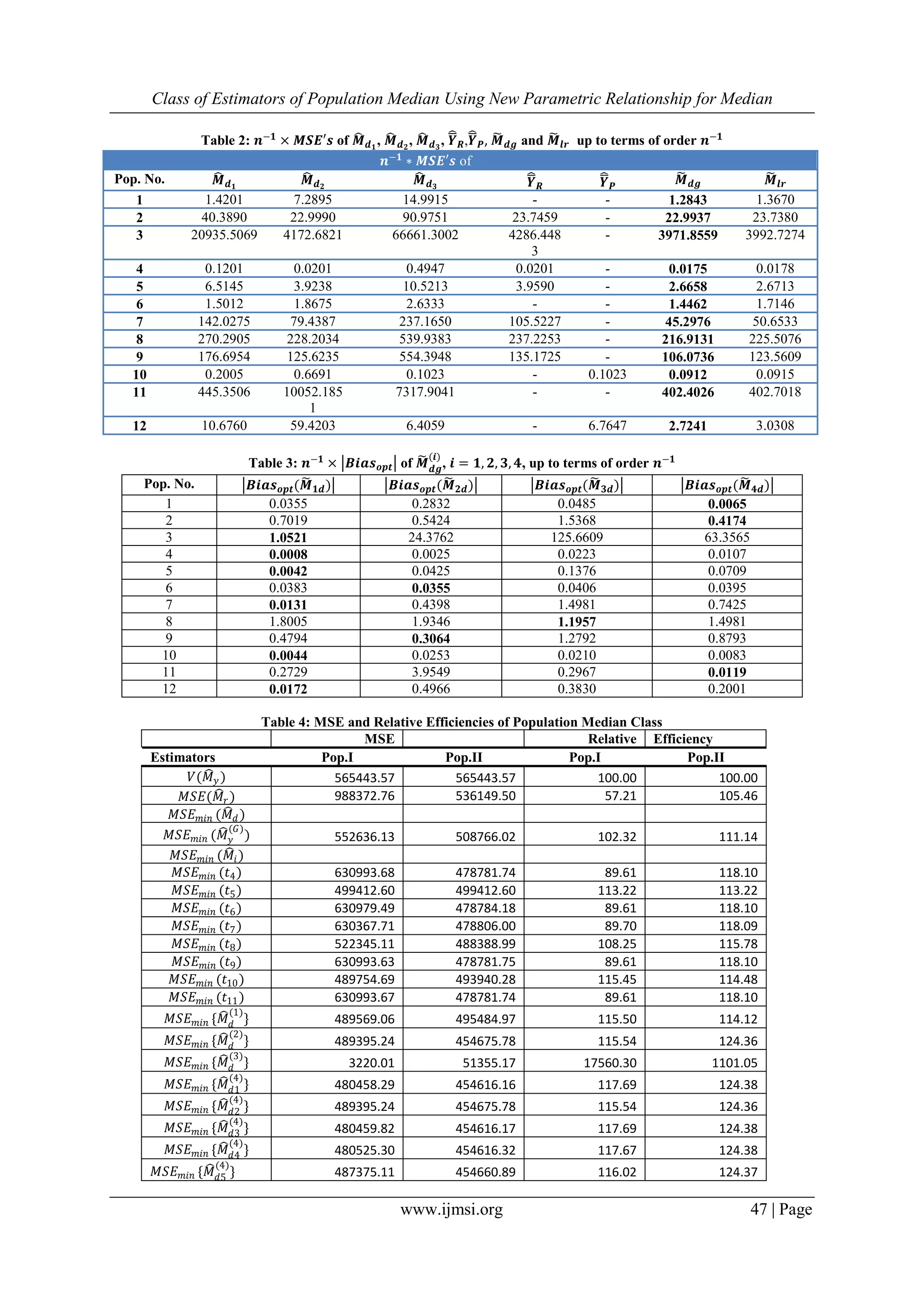
From table 2, in which we compared the estimators of similar type, we observe that, upto the terms of order
𝑛−1,𝑀𝑆𝐸 𝑚𝑖𝑛 𝑀𝑑𝑔 is less than 𝑀𝑆𝐸 𝑚𝑖𝑛 (𝑀 𝑑1
), 𝑀𝑆𝐸 𝑚𝑖𝑛 (𝑀 𝑑2
), 𝑀𝑆𝐸 𝑚𝑖𝑛 (𝑀 𝑑3
), 𝑀𝑆𝐸(𝑌𝑅), 𝑀𝑆𝐸(𝑌𝑃)and even smaller than
𝑀𝑆𝐸 𝑚𝑖𝑛 (𝑌𝑙𝑟 ), which are very interesting results.
From table 3, it is clearly seen that among all the four important types of estimators, the bias of first sub-class of estimators
𝑀 𝑑𝑔
(1)
, which is of regression type, is less in most of the populations.
From table 4, we can see that the efficiency of the proposed optimum estimator of class 𝑀 𝑑𝑔 is very much high as compare to
estimators of different technique.
VII. CONCLUTION
In this study, when 𝑋 is known then we have proposed the generalized class of estimators of population median
which includes the estimators defined by Sharma et al. (2016). The lower bound for MSE for the class of estimators has been
obtained. To choose optimum estimators w.r.t. MSE and bias, important types of sub-classes of proposed generalized class
are considered. Their optimum biases have been obtained and compared with each other.
Empirically we have shown that the sub-class of regression-type estimators 𝑀 𝑑𝑔
(1)
= 𝑀 𝑑 + 𝛼1 𝑢 − 1 are optimum
estimators of population median w.r.t. bias and MSE, as well as very simple as compared to the exisiting ones.
REFERENCES
[1] Kuk AY, Mak TK (1989) Median estimation in the presence of auxiliary information. Journal of the Royal Statistical Society.
Series B (Methodological), 51(2):261-269.
[2] Mak TK, Kuk AY (1993) A new method for estimating finite-population quantiles using auxiliary information, The Canadian
Journal of Statistics, 21(1):29-38.
[3] Garcı MR, Cebrián AA (2001) On estimating the median from survey data using multiple auxiliary information. Metrika, 54(1):
59-76.
[4] Singh HP, Sidhu SS, Singh S (2006) Median estimation with known interquartile range of auxiliary variable. Int. J. Appl. Math.
Statist, 4:68-80.
[5] Al S, Cingi H (2010) New estimators for the population median in simple random sampling. In: Proceedings of the Tenth Islamic
Countries Conference on Statistical Sciences (ICCS-X):Vol-1, pp 375-383.
[6] Singh HP, Solanki RS (2013) Some Classes of Estimators for the Population Median Using Auxiliary Information.
Communications in Statistics-Theory and Methods, 42(23):4222-4238.
[7] Sharma, M.K., Brar, S.S. & Kaur, H. (2016b). Estimators of population median using new parametric relationship for median.
International Journal of Statistics and Applications, 6(6):368-375.
[8] Sharma, M.K., Brar, S.S. & Kaur, H. (2016a). Class of estimators of population mode using new parametric relationship for
mode. American Journal of Mathematics and Statistics, 6(3), 103-107.
[9] Srivastava, S.K. & Jhajj, H.S. (1983). A class of estimators of the population mean using multi-auxiliary information. Cal. Stat.
Assoc. Bull., 32, 47-56.
[10] Murthy, M. N. (1967). Sampling theory and methods. Statistical Publishing Society, Calcutta.
[11] Chakravarty, I. M., Laha, R. G., & Roy, J. (1967). Handbook of Methods of Applied Statistics: Techniques of Computation,
Descriptive Methods, and Statistical Inference. John Wiley & Sons.
[12] Cochran, W. G. (1999). Sampling Techniques (Vol.3). John Wiley & Sons.
[13] Maddala, G. S., & Lahiri, K. (1992). Introduction to econometrics (Vol. 2). New York: Macmillan.
[14] Gujarati, D. N. (2004). Basic Econometrics.Mc. Graw Hills Pub. Co, New York.

Class of Estimators of Population Median Using New Parametric Relationship for Median

More Related Content

What's hot

Viewers also liked

Similar to Class of Estimators of Population Median Using New Parametric Relationship for Median

Recently uploaded

Class of Estimators of Population Median Using New Parametric Relationship for Median