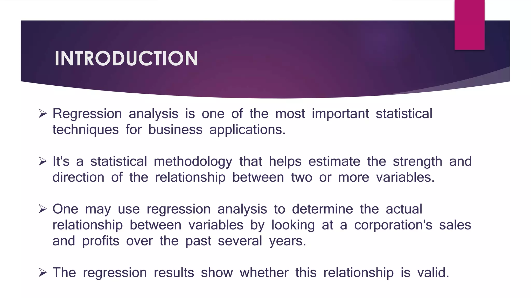
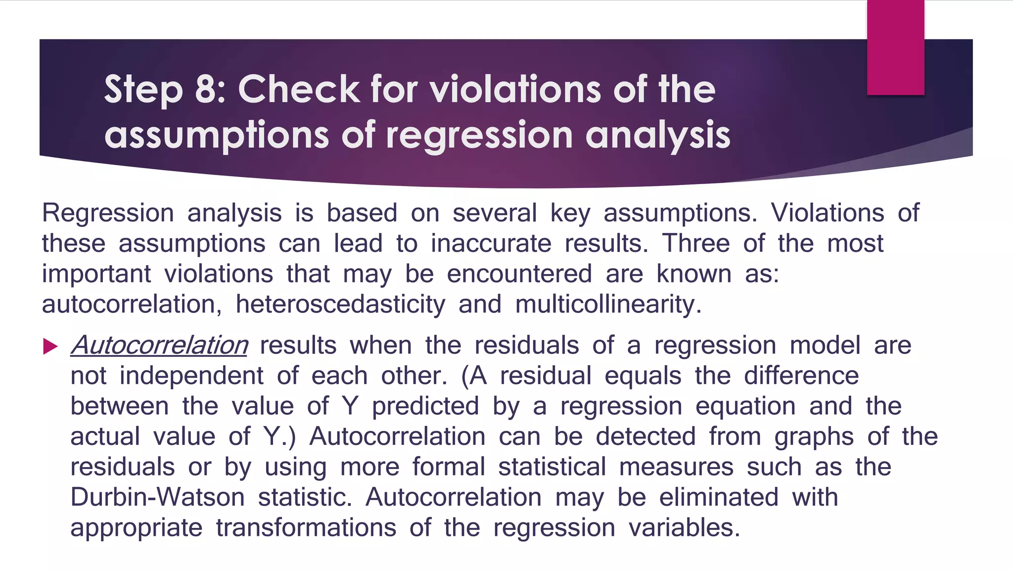
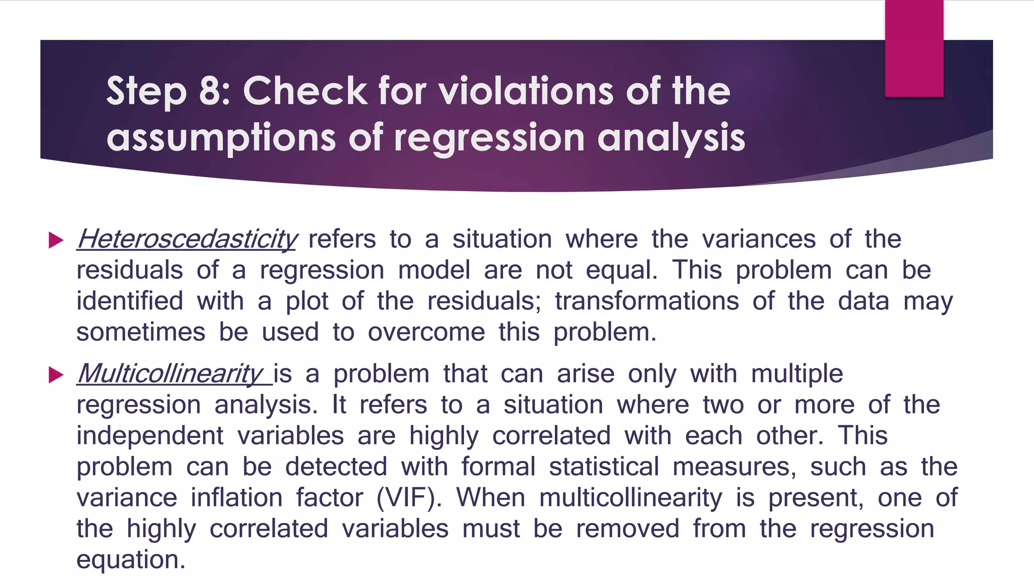
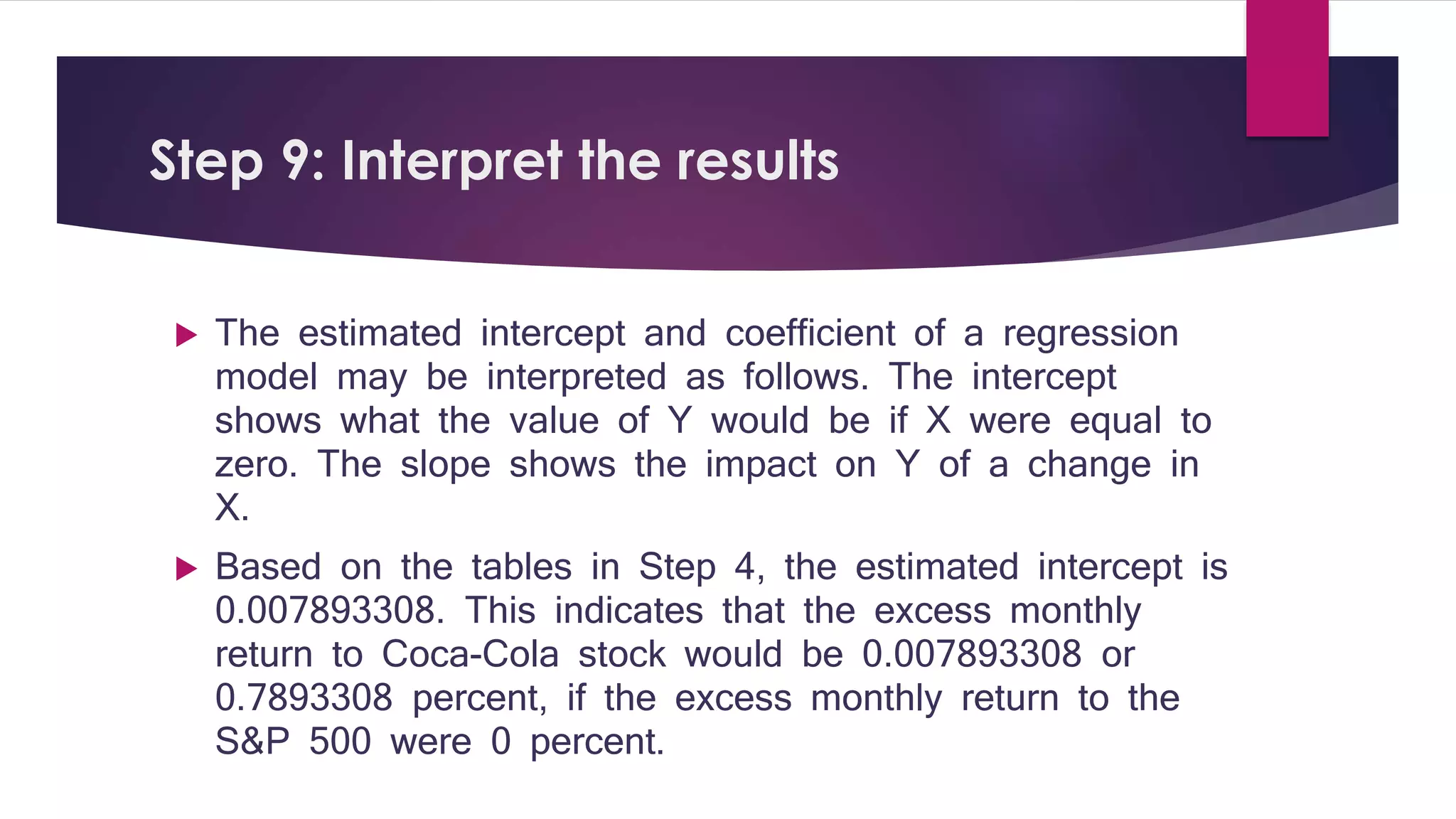
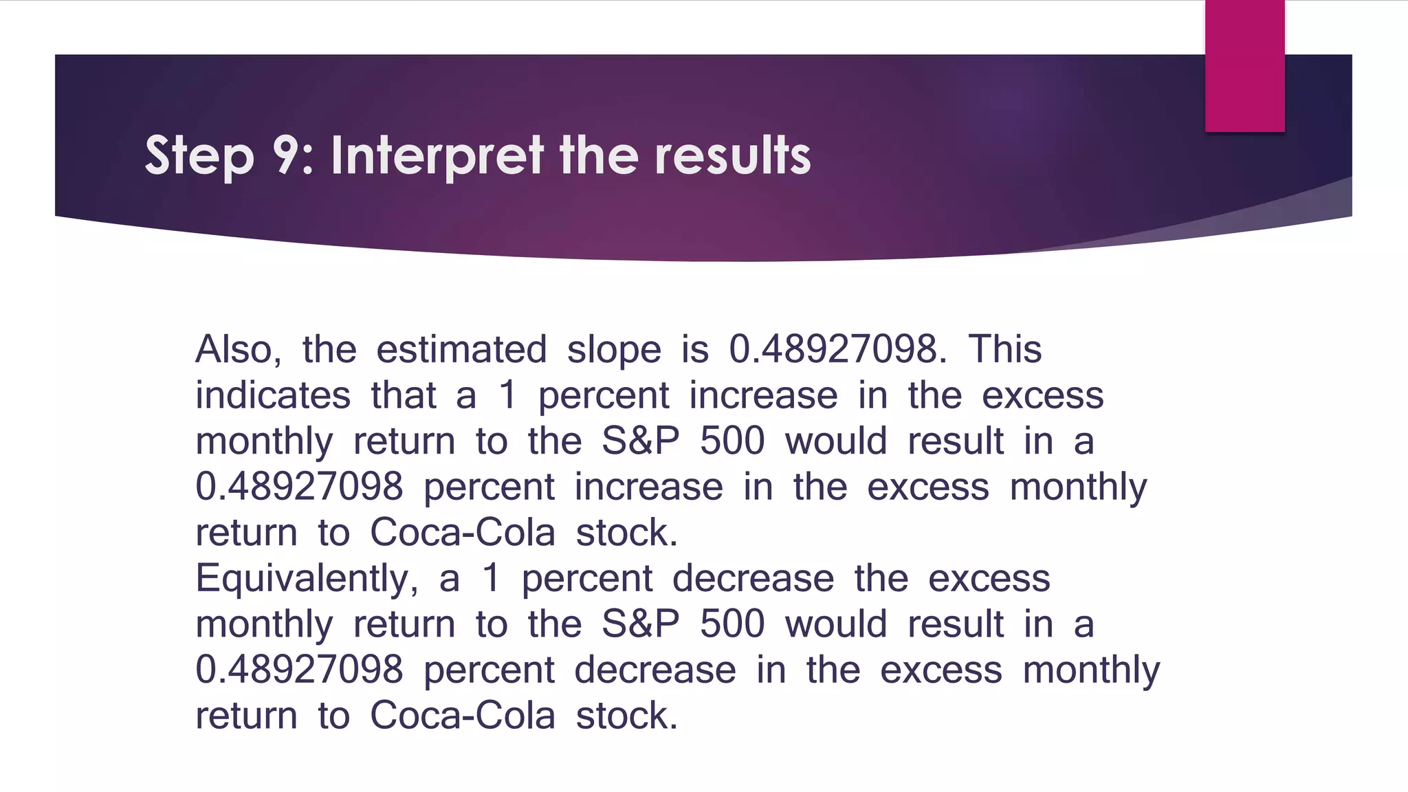
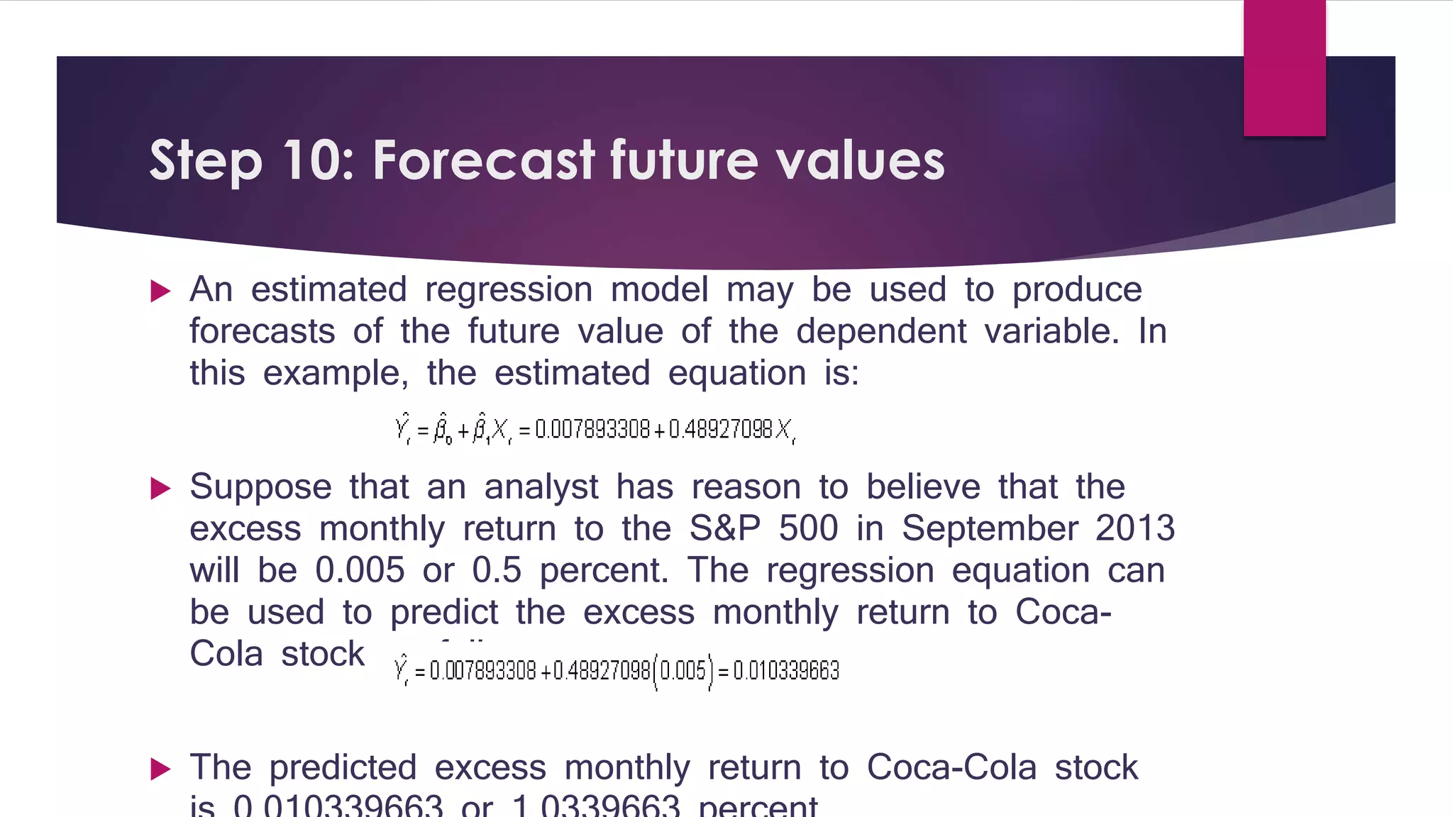
This document provides a summary of regression analysis in 9 steps: 1) Specify dependent and independent variables, 2) Check for linearity with scatter plots, 3) Transform variables if nonlinear, 4) Estimate the regression model, 5) Test the model fit with R2, 6) Perform a joint hypothesis test of the coefficients, 7) Test individual coefficients, 8) Check for violations of assumptions like autocorrelation and heteroscedasticity, 9) Interpret the intercept and slope coefficients. Regression analysis is used to determine relationships between variables and estimate how changes in independents impact dependents.

1. Business Statistics:
Regression Analysis
TO DETERMINE THE VALIDITY OF RELATIONSHIPS
Presented by
Rithish Kumar
Rishabh Chaudhary
Sagar Rathee
Rahul Chauhan

2. INTRODUCTION
 Regression analysis is one of the most important statistical
techniques for business applications.
 It's a statistical methodology that helps estimate the strength and
direction of the relationship between two or more variables.
 One may use regression analysis to determine the actual
relationship between variables by looking at a corporation's sales
and profits over the past several years.
 The regression results show whether this relationship is valid.

3.  Researchers, analysts, portfolio managers, and traders use
regression analysis to estimate historical relationships among
different financial assets. They can then use this information to
develop trading strategies and measure the risk contained in a
portfolio.
 Regression analysis is an indispensable tool for analyzing
relationships between financial variables.
For example, it can:
 Identify the factors that are most responsible for a corporation's
profits
 Determine how much a change in interest rates will impact a
portfolio of bonds

4. The steps used in Implementing a
Regression Model and Analyzing its
Results

5. Step 1: Specify the dependent and
independent variable(s)
 To implement a regression model, it's important to correctly
specify the relationship between the variables being used.
 The value of a dependent variable is assumed to be related
to the value of one or more independent variables .
 A regression model based on a single independent variable
is known as a simple regression model; with two or more
independent variables, the model is known as
a multiple regression model.

6. EXAMPLE:
Suppose that a researcher is investigating
the factors that determine the rate of
inflation. If the researcher believes that the
rate of inflation depends on the growth rate
of the money supply, he may estimate a
regression model using the rate of inflation
as the dependent variable and the growth
rate of the money supply as the
independent variable.

7. Step 2: Check for linearity
 One of the fundamental assumptions of regression analysis
is that the relationship between the dependent and
independent variables is linear.
 One of the quickest ways to verify this is to graph the
variables using a scatter plot . A scatter plot shows the
relationship between two variables with the dependent
variable (Y) on the vertical axis and the independent
variable (X) on the horizontal axis.

8. CASE:
Suppose that an analyst believes that the excess
returns to Coca-Cola stock depend on the excess
returns to the Standard and Poor's (S&P) 500. (The
excess return to a stock equals the actual return
minus the yield on a Treasury bill.) Using monthly
data from September 2008 through August 2013, the
graph on the following slide shows the excess returns
to the S&P 500 on the horizontal axis, whereas the
excess returns to Coca-Cola are on the vertical axis.

9. It can be seen from the scatter plot that this relationship
is approximately linear. Therefore, linear regression may
be used to estimate the relationship between these two
variables.

10. Step 3: Check alternative approaches
if variables are not linear
If the specified dependent (Y) and independent (X) variables don't
have a linear relationship between them, it may be possible
to transform these variables so that they do have a linear
relationship. For example;
 It may be possible that the relationship between the natural logarithm
of Y and X is linear.
 Another possibility is that the relationship between the natural
logarithm of Y and the natural logarithm of X is linear.
 It's also possible that the relationship between the square root of Y
and X is linear.
If these transformations don't produce a linear relationship, alternative
independent variables may be chosen that better explain the value of

11. Step 4: Estimate the model
 The standard linear regression model may be estimated with a
technique known as Ordinary Least Squares(OLS) .
 This results in formulas for the slope and intercept of the
regression equation that "fit" the relationship between the
independent variable (X) and dependent variable (Y) as closely as
possible.
 For example, the tables in the next slide show the results of
estimating a regression model for the excess returns to Coca-Cola
stock and the S&P 500 over the period September 2008 through
August 2013.

12. In this model, the excess returns to Coca-Cola stock are the
dependent variable, while the excess returns to the S&P
500 are the independent variable. Under the Coefficients
column, it can be seen that the estimated intercept of the
regression equation is 0.007893308, and the estimated slope
is 0.48927098.

13. Steps 5: Test the fit of the model using
the coefficient of variation
 The coefficient of variation (also known as R2) is used to determine
how closely a regression model "fits" or explains the relationship
between the independent variable (X) and the dependent variable (Y).
R2 can assume a value between 0 and 1; the closer R2 is to 1, the
better the regression model explains the observed data.
 As shown in the tables from Step 4, the coefficient of variation is
shown as "R-Square"; this equals 0.271795467. The fit isn't particularly
strong. Most likely, the model is incomplete, such as factors other than
the excess returns to the S&P 500 also determine or explain the
excess returns to Coca-Cola stock.
 For a multiple regression model, the adjusted coefficient of determination
is used instead of the coefficient of determination to test the fit of the
regression model.

14. Step 6: Perform a joint hypothesis test
on the coefficients
 A multiple regression equation is used to estimate the
relationship between a dependent variable (Y) and two or more
independent variables (X).
 When implementing a multiple regression model, the overall
quality of the results may be checked with a hypothesis test.
 In this case, the null hypothesis is that all the slope coefficients
of the model equal zero, with the alternative hypothesis that at
least one of the slope coefficients is not equal to zero.
 If this hypothesis can't be rejected, the independent variables
do not explain the value of the dependent variable. If the
hypothesis is rejected, at least one of the independent
variables does explain the value of the dependent variable.

15. Step 7: Perform hypothesis tests on the
individual regression coefficients
 Each estimated coefficient in a regression equation must be tested
to determine if it is statistically significant. If a coefficient is
statistically significant, the corresponding variable helps explain the
value of the dependent variable (Y).
 The null hypothesis that's being tested is that the coefficient equals
zero; if this hypothesis can't be rejected, the corresponding variable
is not statistically significant.
 This type of hypothesis test can be conducted with a p-value (also
known as a probability value .)
 The tables in Step 4 show that the p-value associated with the
slope coefficient is 1.94506 E-05; it can also be written as 1.94506
X 10-5 or 0.0000194506.

16. Step 7: Perform hypothesis tests on the
individual regression coefficients
 The p-value is compared to the level of significance of the
hypothesis test. If the p-value is less than the level of
significance, the null hypothesis that the coefficient equals zero
is rejected; the variable is, therefore, statistically significant.
 In this example, the level of significance is 0.05. The p-value of
0.0000194506 indicates that the slope of this equation is
statistically significant; for example, the excess returns to the
S&P 500 explain the excess returns to Coca-Cola stock.

17. Step 8: Check for violations of the
assumptions of regression analysis
Regression analysis is based on several key assumptions. Violations of
these assumptions can lead to inaccurate results. Three of the most
important violations that may be encountered are known as:
autocorrelation, heteroscedasticity and multicollinearity.
 Autocorrelation results when the residuals of a regression model are
not independent of each other. (A residual equals the difference
between the value of Y predicted by a regression equation and the
actual value of Y.) Autocorrelation can be detected from graphs of the
residuals or by using more formal statistical measures such as the
Durbin-Watson statistic. Autocorrelation may be eliminated with
appropriate transformations of the regression variables.

18. Step 8: Check for violations of the
assumptions of regression analysis
 Heteroscedasticity refers to a situation where the variances of the
residuals of a regression model are not equal. This problem can be
identified with a plot of the residuals; transformations of the data may
sometimes be used to overcome this problem.
 Multicollinearity is a problem that can arise only with multiple
regression analysis. It refers to a situation where two or more of the
independent variables are highly correlated with each other. This
problem can be detected with formal statistical measures, such as the
variance inflation factor (VIF). When multicollinearity is present, one of
the highly correlated variables must be removed from the regression
equation.

19. Step 9: Interpret the results
 The estimated intercept and coefficient of a regression
model may be interpreted as follows. The intercept
shows what the value of Y would be if X were equal to
zero. The slope shows the impact on Y of a change in
X.
 Based on the tables in Step 4, the estimated intercept is
0.007893308. This indicates that the excess monthly
return to Coca-Cola stock would be 0.007893308 or
0.7893308 percent, if the excess monthly return to the
S&P 500 were 0 percent.

20. Step 9: Interpret the results
Also, the estimated slope is 0.48927098. This
indicates that a 1 percent increase in the excess
monthly return to the S&P 500 would result in a
0.48927098 percent increase in the excess monthly
return to Coca-Cola stock.
Equivalently, a 1 percent decrease the excess
monthly return to the S&P 500 would result in a
0.48927098 percent decrease in the excess monthly
return to Coca-Cola stock.

21. Step 10: Forecast future values
 An estimated regression model may be used to produce
forecasts of the future value of the dependent variable. In
this example, the estimated equation is:
 Suppose that an analyst has reason to believe that the
excess monthly return to the S&P 500 in September 2013
will be 0.005 or 0.5 percent. The regression equation can
be used to predict the excess monthly return to Coca-
Cola stock as follows:
 The predicted excess monthly return to Coca-Cola stock
is 0.010339663 or 1.0339663 percent.

22. Sources
 www.google.com/finance?cid=626307
 http://markets.ft.com/research/Markets/Tearsheets/Summary?s=KO:NYQ
 www.thumbcharts.com/100784/KO-vs-S-P-500
 us.spindices.com/indices/equity/sp-500-growth