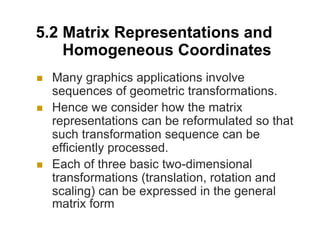
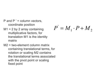
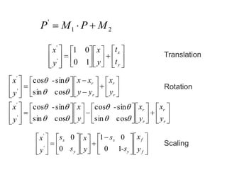
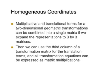
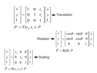
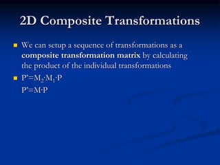
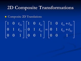
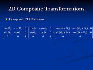
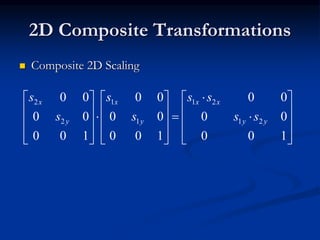
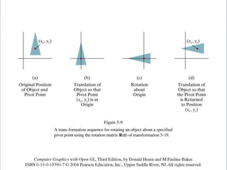
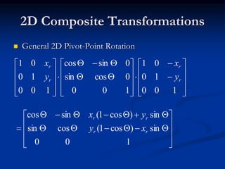
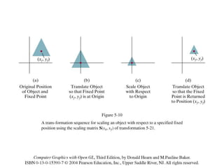
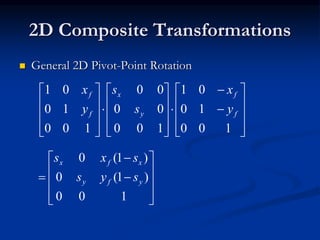
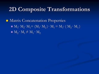
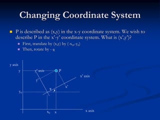
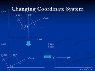
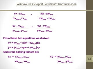
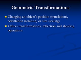
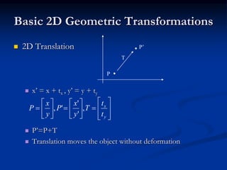
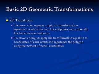
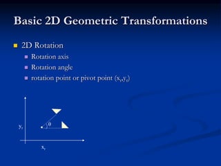
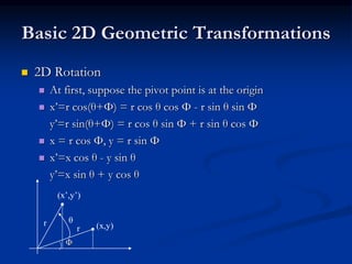
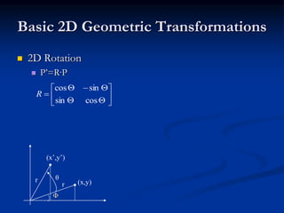
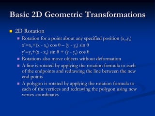
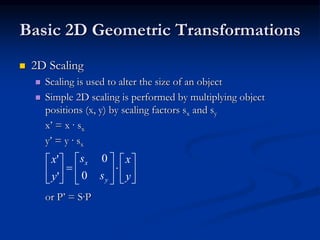
The document discusses 2D geometric transformations including translation, rotation, and scaling. It explains how each transformation can be represented by a matrix and how point coordinates are transformed. It introduces homogeneous coordinates to allow multiple transformations to be combined into a single matrix multiplication by expanding points into 3D vectors. This allows complex sequences of transformations to be applied efficiently in one step.

1. Geometric Transformations
 Changing an object’s position (translation),
orientation (rotation) or size (scaling)
 Others transformations: reflection and shearing
operations

2. Basic 2D Geometric Transformations
 2D Translation
 x’ = x + tx , y’ = y + ty
 P’=P+T
 Translation moves the object without deformation
P
P’
T





















y
x
t
t
T
y
x
P
y
x
P ,
'
'
',

3. Basic 2D Geometric Transformations
 2D Translation
 To move a line segment, apply the transformation
equation to each of the two line endpoints and redraw the
line between new endpoints
 To move a polygon, apply the transformation equation to
coordinates of each vertex and regenerate the polygon
using the new set of vertex coordinates

4. 2D Translation Routine
class wcPt2D {
public:
GLfloat x, y;
};
void translatePolygon (wcPt2D * verts, GLint nVerts, GLfloat tx, GLfloat ty)
{
GLint k;
for (k = 0; k < nVerts; k++) {
verts [k].x = verts [k].x + tx;
verts [k].y = verts [k].y + ty;
}
glBegin (GL_POLYGON);
for (k = 0; k < nVerts; k++)
glVertex2f (verts [k].x, verts [k].y);
glEnd ( );
}

5. Basic 2D Geometric Transformations
 2D Rotation
 Rotation axis
 Rotation angle
 rotation point or pivot point (xr,yr)
yr
xr
θ

6. Basic 2D Geometric Transformations
 2D Rotation
 At first, suppose the pivot point is at the origin
 x’=r cos(θ+Φ) = r cos θ cos Φ - r sin θ sin Φ
y’=r sin(θ+Φ) = r cos θ sin Φ + r sin θ cos Φ
 x = r cos Φ, y = r sin Φ
 x’=x cos θ - y sin θ
y’=x sin θ + y cos θ
Φ
(x,y)r
r θ
(x’,y’)

7. Basic 2D Geometric Transformations
 2D Rotation
 P’=R·P
Φ
(x,y)r
r θ
(x’,y’)









cossin
sincos
R

8. Basic 2D Geometric Transformations
 2D Rotation
 Rotation for a point about any specified position (xr,yr)
x’=xr+(x - xr) cos θ – (y - yr) sin θ
y’=yr+(x - xr) sin θ + (y - yr) cos θ
 Rotations also move objects without deformation
 A line is rotated by applying the rotation formula to each
of the endpoints and redrawing the line between the new
end points
 A polygon is rotated by applying the rotation formula to
each of the vertices and redrawing the polygon using new
vertex coordinates

9. 2D Rotation Routine
class wcPt2D {
public:
GLfloat x, y;
};
void rotatePolygon (wcPt2D * verts, GLint nVerts, wcPt2D pivPt, GLdouble theta)
{
wcPt2D * vertsRot;
GLint k;
for (k = 0; k < nVerts; k++) {
vertsRot [k].x = pivPt.x + (verts [k].x - pivPt.x) * cos (theta) - (verts [k].y - pivPt.y) * sin (theta);
vertsRot [k].y = pivPt.y + (verts [k].x - pivPt.x) * sin (theta) + (verts [k].y - pivPt.y) * cos (theta);
}
glBegin (GL_POLYGON);
for (k = 0; k < nVerts; k++)
glVertex2f (vertsRot [k].x, vertsRot [k].y);
glEnd ( );
}

10. Basic 2D Geometric Transformations
 2D Scaling
 Scaling is used to alter the size of an object
 Simple 2D scaling is performed by multiplying object
positions (x, y) by scaling factors sx and sy
x’ = x · sx
y’ = y · sx
or P’ = S·P


















y
x
s
s
y
x
y
x
0
0
'
'

11. Basic 2D Geometric Transformations
 2D Scaling
 Any positive value can be used as scaling factor
 Values less than 1 reduce the size of the object
 Values greater than 1 enlarge the object
 If scaling factor is 1 then the object stays unchanged
 If sx = sy , we call it uniform scaling
 If scaling factor <1, then the object moves closer to the origin
and If scaling factor >1, then the object moves farther from the
origin
x’ x

12. Basic 2D Geometric Transformations
 2D Scaling
 We can control the location of the scaled object by
choosing a position called the fixed point (xf,yf)
x’ – xf = (x – xf) sx y’ – yf = (y – yf) sy
x’=x · sx + xf (1 – sx)
y’=y · sy + yf (1 – sy)
 Polygons are scaled by applying the above formula to each
vertex, then regenerating the polygon using the
transformed vertices

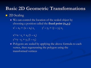
13. 2D Scaling Routine
class wcPt2D {
public:
GLfloat x, y;
};
void scalePolygon (wcPt2D * verts, GLint nVerts, wcPt2D fixedPt, GLfloat sx,
GLfloat sy)
{
wcPt2D vertsNew;
GLint k;
for (k = 0; k < n; k++) {
vertsNew [k].x = verts [k].x * sx + fixedPt.x * (1 - sx);
vertsNew [k].y = verts [k].y * sy + fixedPt.y * (1 - sy);
}
glBegin (GL_POLYGON);
for (k = 0; k < n; k++)
glVertex2v (vertsNew [k].x, vertsNew [k].y);
glEnd ( );
}

14. 5.2 Matrix Representations and
Homogeneous Coordinates
 Many graphics applications involve
sequences of geometric transformations.
 Hence we consider how the matrix
representations can be reformulated so that
such transformation sequence can be
efficiently processed.
 Each of three basic two-dimensional
transformations (translation, rotation and
scaling) can be expressed in the general
matrix form

15. P and P ’ = column vectors,
coordinate position
M1 = 2 by 2 array containing
multiplicative factors, for
translation M1 is the identity
matrix
M2 = two-element column matrix
containing translational terms, for
rotation or scaling M2 contains
the translational terms associated
with the pivot point or scaling
fixed point
21
'
MPMP 

16. 


























y
x
t
t
y
x
y
x
10
01
'
'




































































r
r
r
r
r
r
r
r
y
x
y
x
y
x
y
x
y
x
yy
xx
y
x






cossin
sin-cos
cossin
sin-cos
cossin
sin-cos
'
'
'
'













 





















f
f
y
x
y
x
y
x
-s
s
y
x
s
s
y
x
10
01
0
0
'
'
21
'
MPMP 
Translation
Rotation
Scaling

17.  To produce a sequence of transformations
such as scaling followed by rotation then
translation, we could calculate the
transformed coordinates one step at a time.
 A more efficient approach is to combine the
transformations so that the final coordinate
positions are obtained directly from the
initial coordinates, without calculating
intermediate coordinate values.

18. Homogeneous Coordinates
 Multiplicative and translational terms for a
two-dimensional geometric transformations
can be combined into a single matrix if we
expand the representations to 3 by 3
matrices.
 Then we can use the third column of a
transformation matrix for the translation
terms, and all transformation equations can
be expressed as matrix multiplications.

19.  But to do so, we also need to expand the
matrix representation for a two-dimensional
coordinate position to a three-element column
matrix.
 A standard technique for accomplishing this
is to expand each two-dimensional
coordinate-position representation (x,y) to a
three-element representation (xh,yh,h), called
homogeneous coordinates, where the
homogeneous parameter h is a nonzero
value such that
,
h
y
y
h
x
x hh


20.  A convenient choice is simply to set h=1.
 Each two-dimensional position is then
represented with homogeneous coordinate
(x,y,1).
 The term “homogeneous coordinates” is
used in mathematics to refer to the effect of
this representation on Cartesian equations.

22. PttTP
y
x
t
t
y
x
yx
y
x
































),(
1100
10
01
1
'
'
'
PRP
y
x
y
x
































)(
1100
0cossin
0sin-cos
1
'
'
'



PssSP
y
x
s
s
y
x
yx
y
x
































),(
1100
00
00
1
'
'
'
Translation
Rotation
Scaling

23. 2D Composite Transformations
 We can setup a sequence of transformations as a
composite transformation matrix by calculating
the product of the individual transformations
 P’=M2·M1·P
P’=M·P

24. 2D Composite Transformations
 Composite 2D Translations


































100
10
01
100
10
01
100
10
01
21
21
1
1
2
2
yy
xx
y
x
y
x
tt
tt
t
t
t
t

25. 2D Composite Transformations
 Composite 2D Rotations






































100
0)cos()sin(
0)sin()cos(
100
0cossin
0sincos
100
0cossin
0sincos
2121
2121
11
11
22
22

26. 2D Composite Transformations
 Composite 2D Scaling


































100
00
00
100
00
00
100
00
00
21
21
1
1
2
2
yy
xx
y
x
y
x
ss
ss
s
s
s
s

28. 2D Composite Transformations
 General 2D Pivot-Point Rotation




































100
10
01
100
0cossin
0sincos
100
10
01
r
r
r
r
y
x
y
x













100
sin)cos1(cossin
sin)cos1(sincos
rr
rr
xy
yx

30. 2D Composite Transformations
 General 2D Pivot-Point Rotation


































100
10
01
100
00
00
100
10
01
f
f
y
x
f
f
y
x
s
s
y
x













100
)1(0
)1(0
yfy
xfx
sys
sxs

31. 2D Composite Transformations
 Matrix Concatenation Properties
 M3· M2· M1= (M3· M2 ) · M1 = M3· ( M2 · M1 )
 M2 · M1 ≠ M1 · M2

33. Other Two Dimensional
Transformations
 Reflection
 Transformation that produces a mirror image of an
object
y
x

34.  Reflection
 Image is generated relative to an axis of reflection by
rotating the object 180° about the reflection axis
 Reflection about the line y=0 (the x axis)











100
010
001

35. Other Two Dimensional
Transformations
 Reflection
 Reflection about the line x=0 (the y axis)
 Reflection about the origin










100
010
001












100
010
001

36. Other Two Dimensional
Transformations
 Shear
 Transformation that distorts the shape of an object
such that the transformed shape appears as the
object was composed of internal layers that had been
caused to slide over each other
y
x
(0,1) (1,1)
(1,0)(0,0)
y
x
(2,1) (3,1)
(1,0)(0,0)
shx=2

37. Other Two Dimensional
Transformations
 Shear
 An x-direction shear relative to the x axis
 An y-direction shear relative to the y axis










100
01
001
ysh










100
010
01 xsh
yy
yshxx x


'
'

38. Changing Coordinate System
 P is described as (x,y) in the x-y coordinate system. We wish to
describe P in the x’-y’ coordinate system. What is (x’,y’)?
 First, translate by (x,y) by (-x0,-y0)
 Then, rotate by - q
y axis
x axis
y’ axis
x’ axis
P
y’
x’
x
y
q
y0
x0

39. Changing Coordinate Systemy axis
x axis
y’ axis
x’ axis
P
y’
x’
x
y
q
y axis
y’ axis
x’ axis
P
y’
x’q
y axis/
y’ axis
x axis/x’ axis
P
x’
y’

40. 2D Viewing
 Which part of a picture is to be displayed
 clipping window or world window or viewing
window
 Where that part will be displayed on the display
device
 viewport

41. 2D Viewing
 Clipping window selects what we want to see
 Viewport indicates where it is to be viewed on
the output device
 Usually, clipping windows and viewport are
rectangles

42. 2D Viewing Pipeline
(from Donald Hearn and Pauline Baker)

43. 2D Viewing Pipeline
 2D viewing pipeline
 Construct world-coordinate scene using modeling-
coordinate transformations
 Convert world-coordinates to viewing coordinates
 Transform viewing-coordinates to normalized-
coordinates (ex: between 0 and 1, or between -1 and
1)
 Map normalized-coordinates to device-coordinates.

44. 2D Viewing Pipeline
(from Donald Hearn and Pauline Baker)

45. Transform the square and
the models to the device
coordinates in the display
viewport.
in the modeling
coordinates:
Specify a window Transform the window
and the models to the
area to be displayed
normalized coordinates.
Clip against the square
Xmodeling
Ymodeling
Xnormalized
Ynormalized
Xdevice
Ydevice
The 2D Viewing Pipeline
S(2/width, 2/height);
T(-center);
Trans(models);
// normalized models
// glOrtho()
Clipping();
// clipped models
T(Center);
S(With/2, Height/2);
Trans(models);
// device models
//glViewport()

46. ViewingTransformation
46
 Viewing transformation is the mapping of a part of a world-
coordinate scene to device coordinates.
 In 2D (two dimensional) viewing transformation is simply
referred as the window-to-viewport transformation or the
windowing transformation.
 Mapping a window onto a viewport involves converting from
one coordinate system to another.
 If the window and viewport are in standard position, this just
 involves translation and scaling.
 if the window and/or viewport are not in standard, then
extra transformation which is rotation is required.

47. ViewingTransformation
47
0
1
1
x-world
y-world
window window
Normalised deviceworld
y-view
x-view

48. Window-To-ViewportCoordinateTransformation
48
Window-to-Viewport transformation

49. Window-To-ViewportCoordinateTransformation
49
.
XWmax
YWmax
XWmin
YWmin
XVmaxXVmin
YVmax
YVmin
xw,yw
xv,yv

50. Window-To-ViewportCoordinateTransformation
50
xv - xvmin = xw - xwmin
xvmax - xvmin xwmax - xwmin
yv – yvmin = yw - ywmin
yvmax – yvmin ywmax - ywmin
From these two equations we derived
xv = xvmin + (xw – xwmin)sx
yv = yvmin + (yw – ywmin)sy
where the scaling factors are
sx = xvmax – xvmin sy = yvmax - yvmin
xwmax – xwmin ywmax - ywmin

51. Window-To-ViewportCoordinateTransformation
51
The sequence of transformations are:
1. Perform a scaling transformation using a
fixed-point position of (xwmin,ywmin) that
scales the window area to the size of the
viewport.
2. Translate the scaled window area to the
position of the viewport.

52. Window-To-ViewportCoordinateTransformation
52
 Relative proportions of objects are maintained if the scaling
factors are the same (sx = sy). Otherwise, world objects will be
stretched or contracted in either x or y direction when displayed
on output device.
 How about character strings when map to viewport?
 maintains a constant character size (apply when
standard character fonts cannot be changed).
 If character size can be changed, then windowed will be
applied like other primitives.
 For characters formed with line segments, the mapping
to viewport is carried through sequence of line
transformations .

53. 2001. 7. 13 53
Two-Dimensional Viewing Functions (1/2)
• Definition about a viewing reference system
– evaluateViewOrientationMatrix (x0, y0, xV, yV, error, viewMatrix)
• Setting up the elements of a window-to-viewport mapping
matrix
– setviewRepresentation (ws, viewIndex, viewMatrix, viewMap-
pingMatrix, xclipmin, xclipmin, xclipmin, xclipmin, clipxy)
• Storing combinations of viewing and window-viewport
mappings for various workstations in a viewing table
– evaluateViewMappingMatrix (xwmin, xwmax, ywmin, ywmax,
xvmin, xvmax, yvmin, yvmax, error, viewMappingMatrix)

54. 2001. 7. 13 54
Two-Dimensional Viewing Functions (2/2)
• Selection of a paticular set of options from
the viewing table
– setViewIndex (viewIndex)
• Selection of a workstation window-
viewport pair
– setWorkstationWindow (ws, xwsWindmin,
xwsWindmax, ywsWindmin, ywsWindmax)
– setWorkstationViewport (ws, xwsVPortmin,
xwsVPortmax, ywsVPortmin, ywsVPortmax)

55. 2001. 7. 13 55
Clipping Operations
• Clipping
– Any procedure that identifies those portions of a picture
that are either inside or outside of a specified region of
space
• Applied in World Coordinates
• Adapting Primitive Types
– Point
– Line
– Area (or Polygons)
– Curve, Text (omit!!)

56. 2001. 7. 13 56
Point Clipping
• Assuming that the clip window is a
rectangle in standard position
• Saving a point P=(x, y) for display
• Appling Fields
– Particles (explosion, sea foam)
maxmin
maxmin
ywyyw
xwxxw



57. 2001. 7. 13 57
Line Clipping (1/3)
a) Before Clipping b) After Clipping
• Line clipping against a rectangular clip window

58. 2001. 7. 13 58
Line Clipping (2/3)
• Parametric representation of Line segment
with endpoints (x1, y1) and (x2, y2)
• Exterior of the window
– Intersection with outside the range u
• Interior of the window
– Intersection with inside the range u
),yu(yyy
)xu(xxx
121
121


1u0 

59. Example
Polygon Clipping

60. Example
Polygon Clipping

61. Example
Polygon Clipping

62. Case 1
Inside Outside
Polygon
being
clipped
Clip
boundary
s
p:output
4 Cases of Polygon Clipping
Case 2
Inside Outside
s
p
i:output
Case 3
Inside Outside
s
p
(no output)
Case 4
Inside Outside
s
i:first output
p:second output

63. Algorithm
Input vertex P
First Point YesNo
F=P
Does SP intersect
E?
No
Yes
Compute
Intersection Point
I
Output
vertex I
S=P
Is S on left
side of E?
Exit
NO
Yes
Output
vertex S
Close Polygon entry
Does SF
intersect E?
Compute
Intersection I
Yes
Output
vertex I
Exit
No

64. Curve Clipping
Before Clipping After clipping

65. Text Clipping
Before Clipping After clipping

66. Exterior Clipping
Before Clipping After clipping