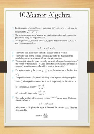
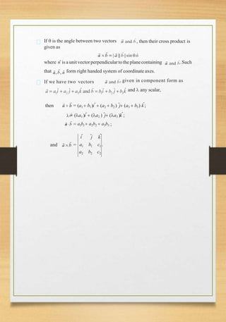
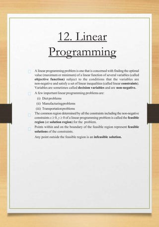
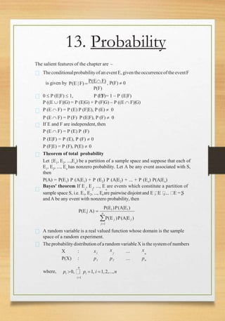
SlideShare a Scribd company logo
Kendriya Vidyalaya
SESSION 2020-21
CLASS 12 MATHEMATICS
FORMULAS
Submitted to:- Submitted by:-
1. Relations and
Functions
◆
◆
◆
◆
◆
◆
◆
◆
◆
◆
◆
◆
◆
Empty relation is the relation R in X given by R =   X × X.
Universal relation is the relation R in X given by R = X × X.
Reflexive relation R in X is a relation with (a, a)  R  a  X.
Symmetric relation R in X is a relation satisfying (a, b)  R implies (b, a)  R.
Transitive relation R in X is a relation satisfying (a, b)  R and (b, c)  R
implies that (a, c) R.
Equivalence relation R in X is a relation which is reflexive, symmetric and
transitive.
Equivalence class [a] containing a  X for an equivalence relation R in X is
the subset of X containing all elements b related toa.
A function f : X  Y is one-one (or injective) if
f (x ) = f (x )  x = x  x , x  X.
1 2 1 2 1 2
A function f : X  Y is onto (or surjective) if given any y  Y,  x  X such
that f (x) = y.
A function f : X  Y is one-one and onto (or bijective), if f is both one-one
and onto.
The composition of functions f : A  B and g : B  C is the function
gof : A  C given by gof (x) = g(f (x))  x  A.
A function f : X  Y is invertible if  g : Y  X such that gof = IX and
fog = IY.
A function f : X  Y is invertible if and only if f is one-one and onto.
◆ Given a finite set X, a function f : X  X is one-one (respectively onto) if and only if f
is onto (respectively one-one). This is the characteristic property of a finite set. This
is not true for infinite set.
◆ A binary operation  on a set A is a function  from A × A to A.
◆ An element e  X is the identity element for binary operation  : X × X  X, if a  e
= a = e  a  a  X.
◆ An element a  X is invertible for binary operation  : X × X  X, if there exists b
 X such that a  b = e = b  a where, e is the identity for the binary operation .
The element b is called inverse of a and is denoted by a–1.
◆ An operation  on X is commutative if a  b = b  a  a, b in X.
◆ An operation  on X is associative if (a  b)  c = a  (b  c) a, b, c in X.
2.INVERSE TRIGONOMETRIC
FUNCTIONS
◆ The domains and ranges (principal value branches) of inverse trigonometric
functionsare given in the followingtable:
Functions Domain Range
(Principal Value Branches)
y = sin–1 x [–1, 1]
  
 2
,
2
y = cos–1 x [–1, 1] [0, ]
y = cosec–1 x R – (–1,1)
  
2
,
2 
– {0}
y = sec–1 x R – (–1, 1)

[0, ] – { }
2
y = tan–1 x R


,

 
 2 2 
y = cot–1 x R (0, )
◆ sin–1x should not be confused with (sin x)–1. In fact (sin x)–1 =
1
sinx
and
similarlyforother trigonometricfunctions.
◆ The value of an inverse trigonometric functions which lies in its principal
value branch is called the principal value of that inverse trigonometric
functions.
For suitable values of domain, wehave
◆
◆
y = sin–1 x  x = sin y
sin (sin–1 x) = x
◆
◆
x = sin y  y = sin–1 x
sin–1 (sin x) = x
◆
1
sin–1 = cosec–1 x ◆ cos–1 (–x) =  – cos–1 x
◆ cos–1
x
1
x
= sec–1
x ◆ cot–1
(–x) =  – cot–1
x
◆
1
x
tan–1
= cot–1
x ◆ sec–1
(–x) =  – sec–1
x
sin–1 (–x) = – sin–1 x tan–1 (–x) = – tan–1 x
◆
◆ 2

tan–1 x + cot–1 x =
◆
◆ cosec–1 (–x) = –cosec–1 x
◆ tan–1x + tan–1y = tan–1
x  y
1 xy ◆ 2

sin–1 x + cos–1 x =
◆ tan–1
x + tan–1
y = tan–1
x  y
1 xy ◆ 2

cosec–1
x + sec–1
x =
◆ 2tan–1 x = sin–1
2x
1 x2 = cos–1
1 x2
1 x2 ◆ 2tan–1x = tan–1
2
2x
1 x
 x  y 
xy
◆ tan–1x + tan–1y =   tan–1

1  , xy>1; x, y> 0
◆ A matrix is an ordered rectangular array of numbers or functions.
◆ A matrix having m rows and n columns is called a matrix of order m × n.
◆ [aij]m × 1 is a column matrix.
◆ [aij]1 × n is a row matrix.
◆ An m × n matrix is a square matrix if m = n.
◆ A = [aij]m × m is a diagonal matrix if aij = 0, when i  j.
3.Matrices
A = [aij]n × n is a scalar matrix if aij = 0, when i  j, aij = k, (k is some
constant), when i = j.
A = [aij]n × n is an identity matrix, if aij = 1, when i = j, aij = 0, when i  j. A
zero matrix has all its elements as zero.
A = [aij] = [bij] = B if (i) A and B are of same order, (ii) aij = bij for all
possible values of i and j.
kA = k[aij]m × n =[k(aij)]m × n
– A = (–1)A
A – B = A + (–1) B
A + B = B + A
(A + B) + C = A + (B + C), where A, B and C are of same order.
k(A + B) = kA + kB, where A and B are of same order, k is constant.
(k + l ) A = kA + lA, where k and l are constant.
◆
◆
◆
◆
◆
◆
◆
◆
◆
◆
◆
◆ If A = [aij]m× n and B = [bjk]n × p , thenAB = C = [cik]m × p, where cik  ∑ aij bjk
j1
(i) A(BC) = (AB)C, (ii) A(B + C) = AB + AC, (iii) (A + B)C = AC + BC
◆
◆
◆
◆
◆
◆
If A = [a ] , then A
or AT = [a ]
ij m × n ji n × m
(i) (
A

)
= A, (ii) (kA)= kA
,(iii) (A + B
)
= A
+ B

, (iv) (AB)= B

A
A is a symmetric
matrix if A
=A.
A is a skew symmetric matrix if A
= – A.
Any square matrix can be represented as the sum of a symmetric and a
skew symmetric matrix.
Elementary operations of a matrix are asfollows:
(i) Ri
 Rj
or Ci
 Cj
(ii) Ri  kRi or Ci  kCi
(iii) Ri  Ri + kRj or Ci  Ci + kCj
If A and B are two square matrices such that AB = BA = I, then B is the
inverse matrix of A and is denoted by A–1 and A is the inverse ofB.
Inverse of a square matrix, if it exists, is unique.
◆
◆
◆
4.Determinants
◆ Determinant of a matrix A = [a11]1× 1 is given by | a11| = a11

a a
◆ Determinant of a matrix A 
a11
 21 22 
a12 
is given by
21 22
a11 a12
A 
a a
= a a – a a
11 22 12 21

◆ Determinantof a matrix A a2 2

a3
a1 b1 c1
b2

b3 c3 
1
c is given by (expandingalongR )
2 2 2 2
3 3 3 3 3 3
b c a c a b
2 2 2 1
b c 1
a 1
a
3 3 3
c b
a b c
a1 b1 c1
A  a b c  a 2
 b 2
 c
For any square matrix A, the |A| satisfy following properties.
◆ |A|= |A|, where A
= transpose of A.
◆ If we interchange any two rows (or columns), then sign of determinant
changes.
◆ If any two rows or any two columns are identical or proportional, then value
of determinant iszero.
◆ If we multiplyeach elementof a row or a column of a determinantby constant
k, then value of determinant is multiplied by k.
◆ Multiplying a determinant by k means multiply elements of only one row
(or one column) by k.
◆If A [a ] , then k .A k3
A
◆
ij 33
◆ If elements of a row or a column in a determinant can be expressed as sum
of two or more elements, then the given determinant can be expressed as
sum of two or more determinants.
If to each element of a row or a column of a determinant the equimultiples of
corresponding elements of other rows or columns are added, then value of
determinant remains same.
◆ Area of a triangle with vertices (x1
, y1
), (x2
, y2
) and (x3
, y3
) is given by
2 2
2
x3 y3
x1 y1 1
 
1
x y 1
1
Minor of an element aij of the determinant of matrix A is the determinant
ij
obtained by deleting ith
row and jth
column and denoted by M .
Cofactor of a of given by A = (– 1)i + j
M
ij ij ij
◆
◆
◆ Valueof determinantof a matrixAis obtainedby sum of productof elements
of a row (or a column) with corresponding cofactors. Forexample,
A = a11 A11 + a12 A12 + a13 A13.
◆ If elements of one row (or column) are multiplied with cofactors of elements
of any other row (or column), then their sum is zero. For example, a11 A21 + a12
A + a A = 0
◆ a a
22 13 23
a11 a12 a13 
,
If A  a
 21 22 23
a31 a32 a33
12 22
A11 A21 A31 
 32 
A13 A23 A33 
ij
then adj A  A A A  , where A is
cofactor of aij
◆
◆
◆
A (adj A) = (adj A) A = |A| I, where A is square matrix of order n.
A square matrix A is said to be singular or non-singular according as
|A| = 0 or |A|  0.
If AB = BA = I, where B is square matrix, then B is called inverse of A.
Also A–1 = B or B–1 = A and hence (A–1)–1 = A.
A square matrixAhas inverse if and only ifA is non-singular.
A–1

1
(adj A)
A
◆
◆
◆ If a1 x + b1 y + c1 z = d1 a2 x
+ b2 y + c2 z = d2 a3 x +
b3 y + c3 z = d3,
b3
then these equations can be written as A X = B, where
a1 b1 c1  x d1 
b c ,X= y and B= d 
A a 2 2   
z
 2
a3 c3 
 2 
d3
◆ Unique solution of equation AX = B is given by X = A–1 B, where A  0.
◆ A system of equation is consistent or inconsistent according as its solution
exists or not.
◆ For a square matrixA in matrix equationAX = B
(i) |A|  0, there exists unique solution
(ii) |A| = 0 and (adj A) B  0, then there exists no solution
(iii)|A| = 0 and (adj A) B = 0, then system may or may not be consistent.
.
5.Continuity and
Differentiability
◆ A real valued function is continuous at a point in its domain if the limit of the
function at that point equals the value of the function at that point. A function
is continuous if it is continuous on the whole of its domin.
◆ Sum, difference, product and quotient of continuous functions are continuous.
i.e., if f and g are continuous functions,then
(f ± g) (x) = f (x) ± g (x) is continuous.
(f . g) (x) = f (x) . g (x) is continuous.
g(x)
f
(x) 
f (x)
(wherever g (x)  0) is continuous.
g
◆ Every differentiable function is continuous, but the converse is not true.
◆ Chain rule is rule to differentiate composites of functions. If f = v o u, t = u (x)
and if both
dt
and
dv
existthen
dx dt
df

dv

dt
dx dt dx
◆ Following are some of the standard derivatives (in appropriate domains):
6. Application of
Derivatives
◆ If a quantity y varies with another quantity x, satisfying some rule y  f (x),
Alternatively, if f (x) 0 for each x in (a, b)
(b) decreasing on (a,b) if
x < x in (a, b)  f (x )  f (x ) for all x , x  (a, b).
1 2 1 2 1 2
(c) constant in (a, b), if f (x) = c for all x  (a, b), where c is a constant.
◆ The equation of the tangent at (x0
, y0
) to the curve y = f (x) is given by
y  y  dy 
dx
0 0
(x0 ,y0 )
(x  x )
◆ dx 0 0
dy
If does not exist at the point ( x , y ) , then the tangent at this point is
parallel to the y-axis and its equation is x = x0.
◆ 0
0
dxx x
If tangent to a curve y = f (x) at x = x is parallel to x-axis, then
dy 
  0.
◆ Equation of the normal to the curve y = f (x) at a point ( x0 , y0 ) is given by
1
0 0
dx (x , y )
y  y0 
dy
(x x0 )
◆ dx 0 0 0
dy
If at the point ( x , y ) is zero, then equation of the normal is x = x.
dx 0 0
◆ If
dy
at the point ( x , y ) does not exist, then the normal is parallel tox-axis
and its equation is y = y0.
◆ Let y = f (x), x be a small increment in x and y be the increment in y
corresponding to the increment in x, i.e., y = f (x + x) – f (x). Then dy
givenby
dy  f (x)dxor dy  

dy 
x .
◆
 dx
isa good approximationofy when dx  x is relativelysmalland we denote
it by dy  y.
A point c in the domain of a function f at which either f (c)= 0 or f is not
differentiable is called a critical point of f.
◆ First Derivative Test Let f be a function defined on an open interval I. Let
f be continuous at a critical point c in I. Then
(ii)
(iii)
(i) If f (x)changes sign from positive to negative as x increases through c,
i.e., if f (x)> 0 at every point sufficiently close to and to the left of c,
and f (x) < 0 at every point sufficiently close to and to the right of c,
then c is a point of local maxima.
If f (x)changes sign from negative to positive as x increases through c,
i.e., if f (x)< 0 at every point sufficiently close to and to the left of c,
and f (x) > 0 at every point sufficiently close to and to the right of c,
then c is a point of local minima.
If f (x)does not change sign as x increases through c, then c is neither a
point of local maxima nor a point of local minima. Infact, such a point
is called point of inflexion.
◆
◆
Second Derivative Test Let f be a function defined on an interval I and
c  I. Let f be twice differentiable at c. Then
(i) x = c is a point of local maxima if f (c)= 0 and f (c) < 0
The values f (c) is local maximum value of f .
(ii) x = c is a point of local minima if f (c)= 0 and f (c) > 0
In this case, f (c) is local minimum value of f.
(iii) The test fails if f (c)= 0 and f (c) = 0.
In this case, we go back to the first derivative test and find whether c is
a pointof maxima,minimaor a pointof inflexion.
Working rulefor findingabsolutemaxima and/orabsoluteminima
Step 1: Find all critical points of f in the interval, i.e., find points x where
either f (x)= 0 or f is not differentiable.
Step 2:Take the end points of theinterval.
Step 3:At all these points (listed in Step 1 and 2), calculate the values of f .
Step 4: Identify the maximum and minimum values of f out of the values
calculated in Step 3. This maximum value will be the absolute maximum
value of f and the minimum value will be the absolute minimum value of f .
7.Integrals
Some standard integrals
(i) n
x dx
xn1
n1
 C , n  – 1. Particularly, dx  x C

(ii) (iii)
(iv) (v)
sin x dx  – cosx  C
cosec2
x dx  – cot x  C
(vi)
(vii)
cos x dx  sin x  C
sec2
x dx  tan x  C
sec x tan x dx  secx  C
cosec x cot x dx  – cosec x  C (viii)
1 x2

dx
 sin1
x  C
(ix)
1 x2

dx
 cos1
x  C (x)
1 x2

dx
 tan  1
x  C
(xi)
1 x2

dx
  cot 1
x C (xii) ex
dx  ex
C
(xiii)
x ax
loga
 C
 a dx  (xiv)  sec 1
x  C
(xv) 
dx
 cosec 1
x  C (xvi)
dx
x x2
1
1
x
dx  log| x |  C



x x2
1
Integration by partial fractions
Recall that a rational function is ratio of two polynomials of the form P(x) ,
Q(x)
where P(x) and Q (x) are polynomials in x and Q (x)  0. If degree of the
polynomial P (x) is greater than the degree of the polynomial Q (x), then we
may divide P (x) by Q (x) so that
P(x)
 T (x) 
P1(x)
, where T(x) is a
Q(x) Q(x)
polynomial in x and degree of P1 (x) is less than the degree of Q(x). T(x)
being polynomial can be easily integrated.
P (x)
1
Q(x)
can be integratedby
expressing
P1(x)
Q(x)
as the sum of partial fractions of the following type:
1. =
A B

x  a x b
, a  b
2. 2
px q
(x  a) (x b)
px q
(x a)
= 2
A B

x  a (x a)
3. =
A

B

C
x  a x  b x c
4. =
5.
px2
 qx  r
(x  a) (x  b) (x  c)
px2
 qx  r
(x  a)2
(x b)
px2
 qx  r
(x  a) (x2
 bx  c)
=
A

B

C
x  a (x  a)2
x b
A

Bx +C
x  a x2
 bx c
where x2 + bx + c can not be factorised further.
Integration by substitution
A change in the variableof integrationoften reduces an integralto one of the
fundamentalintegrals. The method in which we change the variable to some
othervariableiscalledthemethod ofsubstitution.Whentheintegrandinvolves
some trigonometricfunctions, we use some well known identitiesto find the
integrals. Using substitution technique, we obtain the following standard
integrals.
(ii) cot x dx  log sin x  C
(i)
(iii)
(iv)
tan x dx  log secx  C
sec x dx  log secx  tan x  C
cosecx dx  log cosecx  cot x  C
Integrals of some special functions
(i)  log
dx 1 x  a
C
x2
 a2
2a x a

(ii)  log
dx 1 a  x
 C
a2
 x2
2a a x
 (iii)
x
a
1
 tan C
dx 1
x2
 a2
a

(iv)
x2
a2
dx
 log x  x2
 a2
 C (v)
a
a2
x2
dx
 sin 1 x
C
(vi)
x2
a2
dx
 log |x  x2
 a2
| C
Integration by parts
1
For given functions f and f , we have
2
, i.e., the
integral of the product of two functions = first function × integral of the
second function – integral of {differential coefficient of the first function ×
integral of the second function}. Care must be taken in choosing the first
function and the second function. Obviously, we must take that function as
the second function whose integral is well known to us.
ex
[ f (x)  f 
(x)] dx  ex
f (x) dx  C
Some special types of integrals
2 2 2 2 2 2
x a2
x  a dx  x a  log x  x  a C
2 2
(i)
(ii)
2 2 2 2 2 2
x a2
x  a dx  x a  log x  x  a C
2 2
(iii) 2 2 2 2
x a2
1 x
a  x dx  a x  sin C
2 2 a
(iv) Integrals of the types
ax2
 bx c ax2
 bx c
dx
or
dx
can be
transformed into standard form by expressing
b c b 2
c b2
x  
ax2
+ bx + c = a x2
  a x 
a a 2a a 4a2
px  qdx
or
px q dx
ax  bx c
(v) Integrals of the types 2
ax2
 bx  c
can be
b
x
x
transformed into standard form byexpressing
px  q  A
d
(ax2
 bx  c)  B  A (2ax  b)  B , whereAand B are
dx
determined by comparing coefficients on both sides.
We have defined  a
f (x) dx as the area of the region bounded by thecurve
y = f (x), a  x  b, the x-axis and the ordinates x = a and x = b. Let x be a
given point in [a, b]. Then  a
f (x) dx represents the Area function A (x).
This concept of area functionleads to the FundamentalTheorems of Integral
Calculus.
First fundamental theorem of integral calculus
Let the area function be defined by A(x) =  a
f (x) dx for all x  a, where
the function f is assumed to be continuous on [a, b].ThenA
(x) = f (x) for all
x  [a, b].
Second fundamental theorem of integral calculus
Let f be a continuous function of x defined on the closed interval [a, b] and
dx
d
let F be another functionsuch that F(x)  f (x) for all x in the domain of
 
b b
a
a

f, then f (x) dx  F(x) C  F (b)  F (a) .
This is called the definite integral of f over the range [a, b], where a and b
are called the limits of integration, a being the lower limit and b the
upperlimit.
8.Application of Integrals
b b
d d
The area of the region bounded by the curve y = f (x), x-axis and the lines
x = a and x = b (b > a) is given by the formula: Area   a
ydx  a
f (x)dx .
The area of the region bounded by the curve x =  (y), y-axis and the lines
y = c, y = d is given by the formula: Area c
xdy  c
 (y)dy .
The area of the region enclosed between two curves y = f (x), y = g (x) and
the lines x = a, x = b is given by theformula,
 
b
a

Area f (x)  g(x) dx , where, f(x)  g (x) in [a, b]
If f (x)  g (x) in [a, c] and f (x)  g (x) in [c, b], a < c < b, then
 
c b
a c
Area  f (x) g(x) dx  g(
   x)  f (x)dx.
dx dy
dx
 g (x, y) where, f (x, y) and g(x, y) are homogenous
An equation involving derivatives of the dependent variable with respect to
independent variable (variables) is known as a differential equation.
Order of a differential equation is the order of the highest order derivative
occurringin the differentialequation.
Degree of a differential equation is defined if it is a polynomial equation in its
derivatives.
Degree (when defined) of a differential equation is the highest power (positive
integer only) of the highest order derivative in it.
A function which satisfies the given differential equation is called its solution.
The solution which contains as many arbitrary constants as the order of the
differential equation is called a general solution and the solution free from
arbitraryconstants is called particularsolution.
To form a differential equation from a given function we differentiate the
function successively as many times as the number of arbitrary constants in
the given function and then eliminate the arbitrary constants.
Variable separable method is used to solve such an equation in which variables
can be separated completely i.e. terms containing y should remain with dy
and terms containing x should remain withdx.
A differential equation which can be expressed in the form
dy
 f (x, y) or
functions of degree zero is called a homogeneous differential equation.
A differentialequationofthe form
dy
+Py  Q , where P and Q are constants
dx
or functions of x only is called a first order linear differential equation.
9. Differential Equations
10.Vector Algebra
Positionvectorof a pointP(x, y, z) is given as ,andits
magnitude by x2
 y2
 z2 .
The scalar components of a vector are its direction ratios, and represent its
projections along the respective axes.
The magnitude (r), direction ratios (a, b, c) and direction cosines (l, m, n) of
any vector are related as:
l 
a
, m 
b
, n 
c
r r r
, then their cross product is
If  is the angle between two vectors
given as
where nˆ is a unitvectorperpendicularto the planecontaining .Such
that form right handed system of coordinate axes.
If we have two vectors , given in component form as
and  any scalar,
then = (a1  b1)iˆ (a2  b2 ) ˆj (a3  b3) kˆ;
 = (a1 )iˆ (a2 ) ˆj (a3 )kˆ;
= a1b1 a2b2  a3b3 ;
and =
ˆj kˆ
iˆ
a1 b1 c1 .
a2 b2 c2
12. Linear
Programming
A linear programming problemis one that is concerned with finding the optimal
value (maximum or minimum) of a linear function of several variables (called
objective function) subject to the conditions that the variables are
non-negative and satisfy a set of linear inequalities (called linear constraints).
Variables are sometimes called decision variables and are non-negative.
A few important linearprogramming problems are:
(i) Dietproblems
(ii) Manufacturingproblems
(iii) Transportationproblems
The common region determined by all the constraints including the non-negative
constraints x  0, y  0 of a linear programming problem is called the feasible
region (or solution region) for the problem.
Points within and on the boundary of the feasible region represent feasible
solutions of the constraints.
Any point outside the feasible region is an infeasible solution.
Any point in the feasible region that gives the optimal value (maximum or
minimum) of the objective function is called an optimal solution.
The following Theorems are fundamental in solving linear programming
problems:
Theorem 1 Let R be the feasible region (convex polygon) for a linear
programming problem and let Z = ax + by be the objective function. When Z
has an optimal value (maximum or minimum), where the variables x and y
are subject to constraints described by linear inequalities, this optimal value
must occur at a corner point (vertex) of the feasible region.
Theorem 2 Let R be the feasible region for a linear programming problem,
and let Z = ax + by be the objective function. If R is bounded, then the
objective function Z has both a maximum and a minimum value on R and
each of these occurs at a corner point (vertex) of R.
If the feasible region is unbounded, then a maximum or a minimum may not
exist. However, if it exists, it must occur at a corner point of R.
Corner point method for solving a linear programming problem. The method
comprisesof the following steps:
(i) Findthefeasibleregionofthelinearprogrammingproblemanddetermine
its corner points (vertices).
(ii) Evaluate the objective function Z = ax + by at each corner point. Let M
and m respectively be the largest and smallest values at thesepoints.
(iii) If thefeasibleregionisbounded,M andm respectivelyarethemaximum
and minimumvaluesof theobjectivefunction.
If the feasible region is unbounded, then
(i) M is the maximum value of the objective function, if the open half plane
determined by ax + by > M has no point in common with the feasible
region. Otherwise, the objective function has no maximum value.
(ii) m is the minimum value of the objective function, if the open half plane
determined by ax + by < m has no point in common with the feasible
region. Otherwise, the objective function has no minimum value.
If two corner points of the feasible region are both optimal solutions of the
same type, i.e., both produce the same maximum or minimum, then any point
on the line segment joining these two points is also an optimal solution of the
same type.
13. Probability
The salient features of the chapter are –
Theconditionalprobabilityof an eventE, given theoccurrenceof the eventF
is given by P(E | F) 
P(E F) , P(F)  0
P(F)
0  P (E|F)  1, P (E|F)= 1 – P (E|F)
P ((E  F)|G) = P (E|G) + P (F|G) – P ((E  F)|G)
P (E  F) = P (E) P (F|E), P (E)  0
P (E  F) = P (F) P (E|F), P (F)  0
If E and F are independent, then
P (E  F) = P (E) P (F)
P (E|F) = P (E), P (F)  0
P (F|E) = P (F), P(E)  0
Theorem of total probability
Let {E1, E2, ...,En) be a partition of a sample space and suppose that each of
E1
, E2
, ..., En
has nonzero probability. Let A be any event associated with S,
then
P(A) = P(E1) P (A|E1) + P (E2) P (A|E2) + ... + P (En) P(A|En)
Bayes' theorem If E , E , ..., E are events which constitute a partition of
1 2 n
sample space S, i.e. E , E , ..., E are pairwise disjoint and E E ... E = S
1 2 n 1 2 n
andA be any event with nonzero probability, then
P(Ei )P(A|Ei )
i n
P(E | A) 
P(E j )P(A|E j )
j1
A random variable is a real valued function whose domain is the sample
space of a random experiment.
The probability distribution ofa random variableX is the system of numbers
X : x1
P(X) : p1
x
2
p2
...
...
x
n
pn
n
where, pi 0, pi 1, i 1,2,...,n
i1
Let X be a random variable whose possible values x , x , x , ..., x occur with
1 2 3 n
1 2 3 n
probabilities p , p , p , ... p respectively. The mean of X, denoted by , is
n
the number  xi pi .
i1
The mean of a randomvariableX is alsocalledtheexpectationof X, denoted
by E (X).
Let X be a random variable whose possible values x1, x2, ..., xn occur with
1 2 n
probabilities p(x ), p(x ), ..., p(x ) respectively.
Let  = E(X) be the mean of X. The variance of X, denoted by Var (X) or
x
2
 , is defined as
2
or equivalently  = E (X –) 2
x
The non-negativenumber
is called the standard deviation of the random variable X.
Var (X) = E (X2) – [E(X)]2
Trials of a random experiment are called Bernoulli trials, if they satisfy the
following conditions:
(i) There should be a finite number of trials.
(ii) The trials should be independent.
(iii) Each trial has exactly two outcomes : success or failure.
(iv) The probability of success remains the same in eachtrial.
For Binomial distribution B (n, p), P (X = x) = nC q n–x px, x = 0, 1,..., n
x
(q = 1 – p)

More Related Content

What's hot

chemistry investigatory project on food adulteration
chemistry investigatory project on food adulterationchemistry investigatory project on food adulteration
chemistry investigatory project on food adulteration
appietech
 
Wheatstone Bridge
Wheatstone BridgeWheatstone Bridge
Wheatstone Bridge
Nishchay Saxena
 
cbse 12th chemistry investigatory project
cbse 12th chemistry investigatory project cbse 12th chemistry investigatory project
cbse 12th chemistry investigatory project
NIKHIL DWIVEDI
 
Physics Investigatory Project - Class 12 - Tangent Galvanometer
Physics Investigatory Project - Class 12 - Tangent GalvanometerPhysics Investigatory Project - Class 12 - Tangent Galvanometer
Physics Investigatory Project - Class 12 - Tangent Galvanometer
Dhananjay Dhiman
 
Chemistry Practical Record Full CBSE Class 12
Chemistry Practical Record Full CBSE Class 12 Chemistry Practical Record Full CBSE Class 12
Chemistry Practical Record Full CBSE Class 12
Muhammad Jassim
 
Full wave rectifier Physics Investigatory Project
Full wave rectifier Physics Investigatory ProjectFull wave rectifier Physics Investigatory Project
Full wave rectifier Physics Investigatory Project
Saksham Mittal
 
CBSE Class XII Physics Investigatory Project
CBSE Class XII Physics Investigatory ProjectCBSE Class XII Physics Investigatory Project
CBSE Class XII Physics Investigatory Project
Vaibhav Kandwal
 
XII INVESTIGATORY PHYSICS PROJECT
XII INVESTIGATORY PHYSICS PROJECTXII INVESTIGATORY PHYSICS PROJECT
XII INVESTIGATORY PHYSICS PROJECT
Er Shambhu Chauhan
 
Chemistry Investigation Project (Daniel cell).
Chemistry Investigation Project (Daniel cell).Chemistry Investigation Project (Daniel cell).
Chemistry Investigation Project (Daniel cell).
sanjeebankrishna
 
Maths practical file (class 12)
Maths practical file (class 12)Maths practical file (class 12)
Maths practical file (class 12)
Anushka Rai
 
CLASS 12th PHYSICS PRACTICAL FILE
CLASS 12th PHYSICS PRACTICAL FILECLASS 12th PHYSICS PRACTICAL FILE
CLASS 12th PHYSICS PRACTICAL FILE
Anushka Rai
 
Chemistry project Class 12th ( Rate of evaporation of different liquids )
Chemistry project Class 12th ( Rate of evaporation of different liquids )Chemistry project Class 12th ( Rate of evaporation of different liquids )
Chemistry project Class 12th ( Rate of evaporation of different liquids )
Vidhi Kishor
 
Physics activity file class 12
Physics activity file class 12Physics activity file class 12
Physics activity file class 12
Titiksha Sharma
 
“To estimate the charge induced on each one of the two identical Styrofoam (o...
“To estimate the charge induced on each one of the two identical Styrofoam (o...“To estimate the charge induced on each one of the two identical Styrofoam (o...
“To estimate the charge induced on each one of the two identical Styrofoam (o...
VanshPatil7
 
Computer science class 12 project on Super Market Billing
Computer science class 12 project on Super Market BillingComputer science class 12 project on Super Market Billing
Computer science class 12 project on Super Market Billing
Harsh Kumar
 
Rectifier class 12th physics investigatory project
Rectifier class 12th physics investigatory projectRectifier class 12th physics investigatory project
Rectifier class 12th physics investigatory project
ndaashishk7781
 
Maths Class 12 Probability Project Presentation
Maths Class 12 Probability Project PresentationMaths Class 12 Probability Project Presentation
Maths Class 12 Probability Project Presentation
Aaditya Pandey
 
Computer Science Investigatory Project Class 12
Computer Science Investigatory Project Class 12Computer Science Investigatory Project Class 12
Computer Science Investigatory Project Class 12
Self-employed
 
CLASS 12 PHYSICS PROJECT - Measuring current using halfwave rectifier
CLASS 12 PHYSICS PROJECT - Measuring current using halfwave rectifierCLASS 12 PHYSICS PROJECT - Measuring current using halfwave rectifier
CLASS 12 PHYSICS PROJECT - Measuring current using halfwave rectifier
Mathesh T
 
Study of adulterants in food stuff
Study of adulterants in food stuffStudy of adulterants in food stuff
Study of adulterants in food stuff
Swaroop Puhan
 

What's hot (20)

chemistry investigatory project on food adulteration
chemistry investigatory project on food adulterationchemistry investigatory project on food adulteration
chemistry investigatory project on food adulteration
 
Wheatstone Bridge
Wheatstone BridgeWheatstone Bridge
Wheatstone Bridge
 
cbse 12th chemistry investigatory project
cbse 12th chemistry investigatory project cbse 12th chemistry investigatory project
cbse 12th chemistry investigatory project
 
Physics Investigatory Project - Class 12 - Tangent Galvanometer
Physics Investigatory Project - Class 12 - Tangent GalvanometerPhysics Investigatory Project - Class 12 - Tangent Galvanometer
Physics Investigatory Project - Class 12 - Tangent Galvanometer
 
Chemistry Practical Record Full CBSE Class 12
Chemistry Practical Record Full CBSE Class 12 Chemistry Practical Record Full CBSE Class 12
Chemistry Practical Record Full CBSE Class 12
 
Full wave rectifier Physics Investigatory Project
Full wave rectifier Physics Investigatory ProjectFull wave rectifier Physics Investigatory Project
Full wave rectifier Physics Investigatory Project
 
CBSE Class XII Physics Investigatory Project
CBSE Class XII Physics Investigatory ProjectCBSE Class XII Physics Investigatory Project
CBSE Class XII Physics Investigatory Project
 
XII INVESTIGATORY PHYSICS PROJECT
XII INVESTIGATORY PHYSICS PROJECTXII INVESTIGATORY PHYSICS PROJECT
XII INVESTIGATORY PHYSICS PROJECT
 
Chemistry Investigation Project (Daniel cell).
Chemistry Investigation Project (Daniel cell).Chemistry Investigation Project (Daniel cell).
Chemistry Investigation Project (Daniel cell).
 
Maths practical file (class 12)
Maths practical file (class 12)Maths practical file (class 12)
Maths practical file (class 12)
 
CLASS 12th PHYSICS PRACTICAL FILE
CLASS 12th PHYSICS PRACTICAL FILECLASS 12th PHYSICS PRACTICAL FILE
CLASS 12th PHYSICS PRACTICAL FILE
 
Chemistry project Class 12th ( Rate of evaporation of different liquids )
Chemistry project Class 12th ( Rate of evaporation of different liquids )Chemistry project Class 12th ( Rate of evaporation of different liquids )
Chemistry project Class 12th ( Rate of evaporation of different liquids )
 
Physics activity file class 12
Physics activity file class 12Physics activity file class 12
Physics activity file class 12
 
“To estimate the charge induced on each one of the two identical Styrofoam (o...
“To estimate the charge induced on each one of the two identical Styrofoam (o...“To estimate the charge induced on each one of the two identical Styrofoam (o...
“To estimate the charge induced on each one of the two identical Styrofoam (o...
 
Computer science class 12 project on Super Market Billing
Computer science class 12 project on Super Market BillingComputer science class 12 project on Super Market Billing
Computer science class 12 project on Super Market Billing
 
Rectifier class 12th physics investigatory project
Rectifier class 12th physics investigatory projectRectifier class 12th physics investigatory project
Rectifier class 12th physics investigatory project
 
Maths Class 12 Probability Project Presentation
Maths Class 12 Probability Project PresentationMaths Class 12 Probability Project Presentation
Maths Class 12 Probability Project Presentation
 
Computer Science Investigatory Project Class 12
Computer Science Investigatory Project Class 12Computer Science Investigatory Project Class 12
Computer Science Investigatory Project Class 12
 
CLASS 12 PHYSICS PROJECT - Measuring current using halfwave rectifier
CLASS 12 PHYSICS PROJECT - Measuring current using halfwave rectifierCLASS 12 PHYSICS PROJECT - Measuring current using halfwave rectifier
CLASS 12 PHYSICS PROJECT - Measuring current using halfwave rectifier
 
Study of adulterants in food stuff
Study of adulterants in food stuffStudy of adulterants in food stuff
Study of adulterants in food stuff
 

Similar to CBSE Class 12 Mathematics formulas

Functions for Grade 10
Functions for Grade 10Functions for Grade 10
Functions for Grade 10
Boipelo Radebe
 
Maths-->>Eigenvalues and eigenvectors
Maths-->>Eigenvalues and eigenvectorsMaths-->>Eigenvalues and eigenvectors
Maths-->>Eigenvalues and eigenvectors
Jaydev Kishnani
 
Quadratic functions
Quadratic functionsQuadratic functions
Quadratic functions
Reynaldo San Juan
 
Engg maths k notes(4)
Engg maths k notes(4)Engg maths k notes(4)
Engg maths k notes(4)
Ranjay Kumar
 
Mathematical-Formula-Handbook.pdf-76-watermark.pdf-68.pdf
Mathematical-Formula-Handbook.pdf-76-watermark.pdf-68.pdfMathematical-Formula-Handbook.pdf-76-watermark.pdf-68.pdf
Mathematical-Formula-Handbook.pdf-76-watermark.pdf-68.pdf
9866560321sv
 
Algebric Functions.pdf
Algebric Functions.pdfAlgebric Functions.pdf
Algebric Functions.pdf
MamadArip
 
function
functionfunction
function
som allul
 
237654933 mathematics-t-form-6
237654933 mathematics-t-form-6237654933 mathematics-t-form-6
237654933 mathematics-t-form-6
homeworkping3
 
Basic math including gradient
Basic math including gradientBasic math including gradient
Basic math including gradient
Ramesh Kesavan
 
A New Approach on the Log - Convex Orderings and Integral inequalities of the...
A New Approach on the Log - Convex Orderings and Integral inequalities of the...A New Approach on the Log - Convex Orderings and Integral inequalities of the...
A New Approach on the Log - Convex Orderings and Integral inequalities of the...
inventionjournals
 
Eighan values and diagonalization
Eighan values and diagonalization Eighan values and diagonalization
Eighan values and diagonalization
gandhinagar
 
Functions (Theory)
Functions (Theory)Functions (Theory)
WEEK-4-Piecewise-Function-and-Rational-Function.pptx
WEEK-4-Piecewise-Function-and-Rational-Function.pptxWEEK-4-Piecewise-Function-and-Rational-Function.pptx
WEEK-4-Piecewise-Function-and-Rational-Function.pptx
ExtremelyDarkness2
 
Manyformulas
ManyformulasManyformulas
Manyformulas
techie_govind
 
Lesson 2: A Catalog of Essential Functions (slides)
Lesson 2: A Catalog of Essential Functions (slides)Lesson 2: A Catalog of Essential Functions (slides)
Lesson 2: A Catalog of Essential Functions (slides)
Mel Anthony Pepito
 
Lesson 2: A Catalog of Essential Functions (slides)
Lesson 2: A Catalog of Essential Functions (slides)Lesson 2: A Catalog of Essential Functions (slides)
Lesson 2: A Catalog of Essential Functions (slides)
Matthew Leingang
 
Mathematics - Functions.pdf
Mathematics - Functions.pdfMathematics - Functions.pdf
Mathematics - Functions.pdf
Jihudumie.Com
 
Graphing Quadratic Functions.pptx
Graphing Quadratic Functions.pptxGraphing Quadratic Functions.pptx
Graphing Quadratic Functions.pptx
MaeAnn84
 
JEE+Crash+course+_+Phase+I+_+Session+1+_+Sets+and++Relations+&+Functions+_+7t...
JEE+Crash+course+_+Phase+I+_+Session+1+_+Sets+and++Relations+&+Functions+_+7t...JEE+Crash+course+_+Phase+I+_+Session+1+_+Sets+and++Relations+&+Functions+_+7t...
JEE+Crash+course+_+Phase+I+_+Session+1+_+Sets+and++Relations+&+Functions+_+7t...
7anantsharma7
 
Calculus- Basics
Calculus- BasicsCalculus- Basics
Calculus- Basics
Rabin BK
 

Similar to CBSE Class 12 Mathematics formulas (20)

Functions for Grade 10
Functions for Grade 10Functions for Grade 10
Functions for Grade 10
 
Maths-->>Eigenvalues and eigenvectors
Maths-->>Eigenvalues and eigenvectorsMaths-->>Eigenvalues and eigenvectors
Maths-->>Eigenvalues and eigenvectors
 
Quadratic functions
Quadratic functionsQuadratic functions
Quadratic functions
 
Engg maths k notes(4)
Engg maths k notes(4)Engg maths k notes(4)
Engg maths k notes(4)
 
Mathematical-Formula-Handbook.pdf-76-watermark.pdf-68.pdf
Mathematical-Formula-Handbook.pdf-76-watermark.pdf-68.pdfMathematical-Formula-Handbook.pdf-76-watermark.pdf-68.pdf
Mathematical-Formula-Handbook.pdf-76-watermark.pdf-68.pdf
 
Algebric Functions.pdf
Algebric Functions.pdfAlgebric Functions.pdf
Algebric Functions.pdf
 
function
functionfunction
function
 
237654933 mathematics-t-form-6
237654933 mathematics-t-form-6237654933 mathematics-t-form-6
237654933 mathematics-t-form-6
 
Basic math including gradient
Basic math including gradientBasic math including gradient
Basic math including gradient
 
A New Approach on the Log - Convex Orderings and Integral inequalities of the...
A New Approach on the Log - Convex Orderings and Integral inequalities of the...A New Approach on the Log - Convex Orderings and Integral inequalities of the...
A New Approach on the Log - Convex Orderings and Integral inequalities of the...
 
Eighan values and diagonalization
Eighan values and diagonalization Eighan values and diagonalization
Eighan values and diagonalization
 
Functions (Theory)
Functions (Theory)Functions (Theory)
Functions (Theory)
 
WEEK-4-Piecewise-Function-and-Rational-Function.pptx
WEEK-4-Piecewise-Function-and-Rational-Function.pptxWEEK-4-Piecewise-Function-and-Rational-Function.pptx
WEEK-4-Piecewise-Function-and-Rational-Function.pptx
 
Manyformulas
ManyformulasManyformulas
Manyformulas
 
Lesson 2: A Catalog of Essential Functions (slides)
Lesson 2: A Catalog of Essential Functions (slides)Lesson 2: A Catalog of Essential Functions (slides)
Lesson 2: A Catalog of Essential Functions (slides)
 
Lesson 2: A Catalog of Essential Functions (slides)
Lesson 2: A Catalog of Essential Functions (slides)Lesson 2: A Catalog of Essential Functions (slides)
Lesson 2: A Catalog of Essential Functions (slides)
 
Mathematics - Functions.pdf
Mathematics - Functions.pdfMathematics - Functions.pdf
Mathematics - Functions.pdf
 
Graphing Quadratic Functions.pptx
Graphing Quadratic Functions.pptxGraphing Quadratic Functions.pptx
Graphing Quadratic Functions.pptx
 
JEE+Crash+course+_+Phase+I+_+Session+1+_+Sets+and++Relations+&+Functions+_+7t...
JEE+Crash+course+_+Phase+I+_+Session+1+_+Sets+and++Relations+&+Functions+_+7t...JEE+Crash+course+_+Phase+I+_+Session+1+_+Sets+and++Relations+&+Functions+_+7t...
JEE+Crash+course+_+Phase+I+_+Session+1+_+Sets+and++Relations+&+Functions+_+7t...
 
Calculus- Basics
Calculus- BasicsCalculus- Basics
Calculus- Basics
 

More from Parth Kshirsagar

PNS GHAZI
PNS GHAZIPNS GHAZI
PNS GHAZI
Parth Kshirsagar
 
Population ( class 9 )
Population ( class 9 )    Population ( class 9 )
Population ( class 9 )
Parth Kshirsagar
 
Birlstone
BirlstoneBirlstone
Birlstone
Parth Kshirsagar
 
Bermuda triangle
Bermuda triangleBermuda triangle
Bermuda triangle
Parth Kshirsagar
 
Climate - sst class9
Climate - sst class9 Climate - sst class9
Climate - sst class9
Parth Kshirsagar
 
Diversity in living organisms
Diversity in living organismsDiversity in living organisms
Diversity in living organisms
Parth Kshirsagar
 
WOMEN CASTE AND REFORM
WOMEN CASTE AND REFORM WOMEN CASTE AND REFORM
WOMEN CASTE AND REFORM
Parth Kshirsagar
 

More from Parth Kshirsagar (7)

PNS GHAZI
PNS GHAZIPNS GHAZI
PNS GHAZI
 
Population ( class 9 )
Population ( class 9 )    Population ( class 9 )
Population ( class 9 )
 
Birlstone
BirlstoneBirlstone
Birlstone
 
Bermuda triangle
Bermuda triangleBermuda triangle
Bermuda triangle
 
Climate - sst class9
Climate - sst class9 Climate - sst class9
Climate - sst class9
 
Diversity in living organisms
Diversity in living organismsDiversity in living organisms
Diversity in living organisms
 
WOMEN CASTE AND REFORM
WOMEN CASTE AND REFORM WOMEN CASTE AND REFORM
WOMEN CASTE AND REFORM
 

Recently uploaded

Your Skill Boost Masterclass: Strategies for Effective Upskilling
Your Skill Boost Masterclass: Strategies for Effective UpskillingYour Skill Boost Masterclass: Strategies for Effective Upskilling
Your Skill Boost Masterclass: Strategies for Effective Upskilling
Excellence Foundation for South Sudan
 
How to Make a Field Mandatory in Odoo 17
How to Make a Field Mandatory in Odoo 17How to Make a Field Mandatory in Odoo 17
How to Make a Field Mandatory in Odoo 17
Celine George
 
Chapter 4 - Islamic Financial Institutions in Malaysia.pptx
Chapter 4 - Islamic Financial Institutions in Malaysia.pptxChapter 4 - Islamic Financial Institutions in Malaysia.pptx
Chapter 4 - Islamic Financial Institutions in Malaysia.pptx
Mohd Adib Abd Muin, Senior Lecturer at Universiti Utara Malaysia
 
clinical examination of hip joint (1).pdf
clinical examination of hip joint (1).pdfclinical examination of hip joint (1).pdf
clinical examination of hip joint (1).pdf
Priyankaranawat4
 
Pengantar Penggunaan Flutter - Dart programming language1.pptx
Pengantar Penggunaan Flutter - Dart programming language1.pptxPengantar Penggunaan Flutter - Dart programming language1.pptx
Pengantar Penggunaan Flutter - Dart programming language1.pptx
Fajar Baskoro
 
Pollock and Snow "DEIA in the Scholarly Landscape, Session One: Setting Expec...
Pollock and Snow "DEIA in the Scholarly Landscape, Session One: Setting Expec...Pollock and Snow "DEIA in the Scholarly Landscape, Session One: Setting Expec...
Pollock and Snow "DEIA in the Scholarly Landscape, Session One: Setting Expec...
National Information Standards Organization (NISO)
 
How to Add Chatter in the odoo 17 ERP Module
How to Add Chatter in the odoo 17 ERP ModuleHow to Add Chatter in the odoo 17 ERP Module
How to Add Chatter in the odoo 17 ERP Module
Celine George
 
Exploiting Artificial Intelligence for Empowering Researchers and Faculty, In...
Exploiting Artificial Intelligence for Empowering Researchers and Faculty, In...Exploiting Artificial Intelligence for Empowering Researchers and Faculty, In...
Exploiting Artificial Intelligence for Empowering Researchers and Faculty, In...
Dr. Vinod Kumar Kanvaria
 
Advanced Java[Extra Concepts, Not Difficult].docx
Advanced Java[Extra Concepts, Not Difficult].docxAdvanced Java[Extra Concepts, Not Difficult].docx
Advanced Java[Extra Concepts, Not Difficult].docx
adhitya5119
 
C1 Rubenstein AP HuG xxxxxxxxxxxxxx.pptx
C1 Rubenstein AP HuG xxxxxxxxxxxxxx.pptxC1 Rubenstein AP HuG xxxxxxxxxxxxxx.pptx
C1 Rubenstein AP HuG xxxxxxxxxxxxxx.pptx
mulvey2
 
Digital Artefact 1 - Tiny Home Environmental Design
Digital Artefact 1 - Tiny Home Environmental DesignDigital Artefact 1 - Tiny Home Environmental Design
Digital Artefact 1 - Tiny Home Environmental Design
amberjdewit93
 
BÀI TẬP BỔ TRỢ TIẾNG ANH LỚP 9 CẢ NĂM - GLOBAL SUCCESS - NĂM HỌC 2024-2025 - ...
BÀI TẬP BỔ TRỢ TIẾNG ANH LỚP 9 CẢ NĂM - GLOBAL SUCCESS - NĂM HỌC 2024-2025 - ...BÀI TẬP BỔ TRỢ TIẾNG ANH LỚP 9 CẢ NĂM - GLOBAL SUCCESS - NĂM HỌC 2024-2025 - ...
BÀI TẬP BỔ TRỢ TIẾNG ANH LỚP 9 CẢ NĂM - GLOBAL SUCCESS - NĂM HỌC 2024-2025 - ...
Nguyen Thanh Tu Collection
 
MARY JANE WILSON, A “BOA MÃE” .
MARY JANE WILSON, A “BOA MÃE”           .MARY JANE WILSON, A “BOA MÃE”           .
MARY JANE WILSON, A “BOA MÃE” .
Colégio Santa Teresinha
 
The basics of sentences session 6pptx.pptx
The basics of sentences session 6pptx.pptxThe basics of sentences session 6pptx.pptx
The basics of sentences session 6pptx.pptx
heathfieldcps1
 
South African Journal of Science: Writing with integrity workshop (2024)
South African Journal of Science: Writing with integrity workshop (2024)South African Journal of Science: Writing with integrity workshop (2024)
South African Journal of Science: Writing with integrity workshop (2024)
Academy of Science of South Africa
 
বাংলাদেশ অর্থনৈতিক সমীক্ষা (Economic Review) ২০২৪ UJS App.pdf
বাংলাদেশ অর্থনৈতিক সমীক্ষা (Economic Review) ২০২৪ UJS App.pdfবাংলাদেশ অর্থনৈতিক সমীক্ষা (Economic Review) ২০২৪ UJS App.pdf
বাংলাদেশ অর্থনৈতিক সমীক্ষা (Economic Review) ২০২৪ UJS App.pdf
eBook.com.bd (প্রয়োজনীয় বাংলা বই)
 
RHEOLOGY Physical pharmaceutics-II notes for B.pharm 4th sem students
RHEOLOGY Physical pharmaceutics-II notes for B.pharm 4th sem studentsRHEOLOGY Physical pharmaceutics-II notes for B.pharm 4th sem students
RHEOLOGY Physical pharmaceutics-II notes for B.pharm 4th sem students
Himanshu Rai
 
BBR 2024 Summer Sessions Interview Training
BBR  2024 Summer Sessions Interview TrainingBBR  2024 Summer Sessions Interview Training
BBR 2024 Summer Sessions Interview Training
Katrina Pritchard
 
Hindi varnamala | hindi alphabet PPT.pdf
Hindi varnamala | hindi alphabet PPT.pdfHindi varnamala | hindi alphabet PPT.pdf
Hindi varnamala | hindi alphabet PPT.pdf
Dr. Mulla Adam Ali
 
Leveraging Generative AI to Drive Nonprofit Innovation
Leveraging Generative AI to Drive Nonprofit InnovationLeveraging Generative AI to Drive Nonprofit Innovation
Leveraging Generative AI to Drive Nonprofit Innovation
TechSoup
 

Recently uploaded (20)

Your Skill Boost Masterclass: Strategies for Effective Upskilling
Your Skill Boost Masterclass: Strategies for Effective UpskillingYour Skill Boost Masterclass: Strategies for Effective Upskilling
Your Skill Boost Masterclass: Strategies for Effective Upskilling
 
How to Make a Field Mandatory in Odoo 17
How to Make a Field Mandatory in Odoo 17How to Make a Field Mandatory in Odoo 17
How to Make a Field Mandatory in Odoo 17
 
Chapter 4 - Islamic Financial Institutions in Malaysia.pptx
Chapter 4 - Islamic Financial Institutions in Malaysia.pptxChapter 4 - Islamic Financial Institutions in Malaysia.pptx
Chapter 4 - Islamic Financial Institutions in Malaysia.pptx
 
clinical examination of hip joint (1).pdf
clinical examination of hip joint (1).pdfclinical examination of hip joint (1).pdf
clinical examination of hip joint (1).pdf
 
Pengantar Penggunaan Flutter - Dart programming language1.pptx
Pengantar Penggunaan Flutter - Dart programming language1.pptxPengantar Penggunaan Flutter - Dart programming language1.pptx
Pengantar Penggunaan Flutter - Dart programming language1.pptx
 
Pollock and Snow "DEIA in the Scholarly Landscape, Session One: Setting Expec...
Pollock and Snow "DEIA in the Scholarly Landscape, Session One: Setting Expec...Pollock and Snow "DEIA in the Scholarly Landscape, Session One: Setting Expec...
Pollock and Snow "DEIA in the Scholarly Landscape, Session One: Setting Expec...
 
How to Add Chatter in the odoo 17 ERP Module
How to Add Chatter in the odoo 17 ERP ModuleHow to Add Chatter in the odoo 17 ERP Module
How to Add Chatter in the odoo 17 ERP Module
 
Exploiting Artificial Intelligence for Empowering Researchers and Faculty, In...
Exploiting Artificial Intelligence for Empowering Researchers and Faculty, In...Exploiting Artificial Intelligence for Empowering Researchers and Faculty, In...
Exploiting Artificial Intelligence for Empowering Researchers and Faculty, In...
 
Advanced Java[Extra Concepts, Not Difficult].docx
Advanced Java[Extra Concepts, Not Difficult].docxAdvanced Java[Extra Concepts, Not Difficult].docx
Advanced Java[Extra Concepts, Not Difficult].docx
 
C1 Rubenstein AP HuG xxxxxxxxxxxxxx.pptx
C1 Rubenstein AP HuG xxxxxxxxxxxxxx.pptxC1 Rubenstein AP HuG xxxxxxxxxxxxxx.pptx
C1 Rubenstein AP HuG xxxxxxxxxxxxxx.pptx
 
Digital Artefact 1 - Tiny Home Environmental Design
Digital Artefact 1 - Tiny Home Environmental DesignDigital Artefact 1 - Tiny Home Environmental Design
Digital Artefact 1 - Tiny Home Environmental Design
 
BÀI TẬP BỔ TRỢ TIẾNG ANH LỚP 9 CẢ NĂM - GLOBAL SUCCESS - NĂM HỌC 2024-2025 - ...
BÀI TẬP BỔ TRỢ TIẾNG ANH LỚP 9 CẢ NĂM - GLOBAL SUCCESS - NĂM HỌC 2024-2025 - ...BÀI TẬP BỔ TRỢ TIẾNG ANH LỚP 9 CẢ NĂM - GLOBAL SUCCESS - NĂM HỌC 2024-2025 - ...
BÀI TẬP BỔ TRỢ TIẾNG ANH LỚP 9 CẢ NĂM - GLOBAL SUCCESS - NĂM HỌC 2024-2025 - ...
 
MARY JANE WILSON, A “BOA MÃE” .
MARY JANE WILSON, A “BOA MÃE”           .MARY JANE WILSON, A “BOA MÃE”           .
MARY JANE WILSON, A “BOA MÃE” .
 
The basics of sentences session 6pptx.pptx
The basics of sentences session 6pptx.pptxThe basics of sentences session 6pptx.pptx
The basics of sentences session 6pptx.pptx
 
South African Journal of Science: Writing with integrity workshop (2024)
South African Journal of Science: Writing with integrity workshop (2024)South African Journal of Science: Writing with integrity workshop (2024)
South African Journal of Science: Writing with integrity workshop (2024)
 
বাংলাদেশ অর্থনৈতিক সমীক্ষা (Economic Review) ২০২৪ UJS App.pdf
বাংলাদেশ অর্থনৈতিক সমীক্ষা (Economic Review) ২০২৪ UJS App.pdfবাংলাদেশ অর্থনৈতিক সমীক্ষা (Economic Review) ২০২৪ UJS App.pdf
বাংলাদেশ অর্থনৈতিক সমীক্ষা (Economic Review) ২০২৪ UJS App.pdf
 
RHEOLOGY Physical pharmaceutics-II notes for B.pharm 4th sem students
RHEOLOGY Physical pharmaceutics-II notes for B.pharm 4th sem studentsRHEOLOGY Physical pharmaceutics-II notes for B.pharm 4th sem students
RHEOLOGY Physical pharmaceutics-II notes for B.pharm 4th sem students
 
BBR 2024 Summer Sessions Interview Training
BBR  2024 Summer Sessions Interview TrainingBBR  2024 Summer Sessions Interview Training
BBR 2024 Summer Sessions Interview Training
 
Hindi varnamala | hindi alphabet PPT.pdf
Hindi varnamala | hindi alphabet PPT.pdfHindi varnamala | hindi alphabet PPT.pdf
Hindi varnamala | hindi alphabet PPT.pdf
 
Leveraging Generative AI to Drive Nonprofit Innovation
Leveraging Generative AI to Drive Nonprofit InnovationLeveraging Generative AI to Drive Nonprofit Innovation
Leveraging Generative AI to Drive Nonprofit Innovation
 

CBSE Class 12 Mathematics formulas

  • 1. Kendriya Vidyalaya SESSION 2020-21 CLASS 12 MATHEMATICS FORMULAS Submitted to:- Submitted by:-
  • 2. 1. Relations and Functions ◆ ◆ ◆ ◆ ◆ ◆ ◆ ◆ ◆ ◆ ◆ ◆ ◆ Empty relation is the relation R in X given by R =   X × X. Universal relation is the relation R in X given by R = X × X. Reflexive relation R in X is a relation with (a, a)  R  a  X. Symmetric relation R in X is a relation satisfying (a, b)  R implies (b, a)  R. Transitive relation R in X is a relation satisfying (a, b)  R and (b, c)  R implies that (a, c) R. Equivalence relation R in X is a relation which is reflexive, symmetric and transitive. Equivalence class [a] containing a  X for an equivalence relation R in X is the subset of X containing all elements b related toa. A function f : X  Y is one-one (or injective) if f (x ) = f (x )  x = x  x , x  X. 1 2 1 2 1 2 A function f : X  Y is onto (or surjective) if given any y  Y,  x  X such that f (x) = y. A function f : X  Y is one-one and onto (or bijective), if f is both one-one and onto. The composition of functions f : A  B and g : B  C is the function gof : A  C given by gof (x) = g(f (x))  x  A. A function f : X  Y is invertible if  g : Y  X such that gof = IX and fog = IY. A function f : X  Y is invertible if and only if f is one-one and onto. ◆ Given a finite set X, a function f : X  X is one-one (respectively onto) if and only if f is onto (respectively one-one). This is the characteristic property of a finite set. This is not true for infinite set. ◆ A binary operation  on a set A is a function  from A × A to A. ◆ An element e  X is the identity element for binary operation  : X × X  X, if a  e = a = e  a  a  X. ◆ An element a  X is invertible for binary operation  : X × X  X, if there exists b  X such that a  b = e = b  a where, e is the identity for the binary operation . The element b is called inverse of a and is denoted by a–1. ◆ An operation  on X is commutative if a  b = b  a  a, b in X. ◆ An operation  on X is associative if (a  b)  c = a  (b  c) a, b, c in X.
  • 3. 2.INVERSE TRIGONOMETRIC FUNCTIONS ◆ The domains and ranges (principal value branches) of inverse trigonometric functionsare given in the followingtable: Functions Domain Range (Principal Value Branches) y = sin–1 x [–1, 1]     2 , 2 y = cos–1 x [–1, 1] [0, ] y = cosec–1 x R – (–1,1)    2 , 2  – {0} y = sec–1 x R – (–1, 1)  [0, ] – { } 2 y = tan–1 x R   ,     2 2  y = cot–1 x R (0, ) ◆ sin–1x should not be confused with (sin x)–1. In fact (sin x)–1 = 1 sinx and similarlyforother trigonometricfunctions. ◆ The value of an inverse trigonometric functions which lies in its principal value branch is called the principal value of that inverse trigonometric functions. For suitable values of domain, wehave ◆ ◆ y = sin–1 x  x = sin y sin (sin–1 x) = x ◆ ◆ x = sin y  y = sin–1 x sin–1 (sin x) = x ◆ 1 sin–1 = cosec–1 x ◆ cos–1 (–x) =  – cos–1 x ◆ cos–1 x 1 x = sec–1 x ◆ cot–1 (–x) =  – cot–1 x ◆ 1 x tan–1 = cot–1 x ◆ sec–1 (–x) =  – sec–1 x
  • 4. sin–1 (–x) = – sin–1 x tan–1 (–x) = – tan–1 x ◆ ◆ 2  tan–1 x + cot–1 x = ◆ ◆ cosec–1 (–x) = –cosec–1 x ◆ tan–1x + tan–1y = tan–1 x  y 1 xy ◆ 2  sin–1 x + cos–1 x = ◆ tan–1 x + tan–1 y = tan–1 x  y 1 xy ◆ 2  cosec–1 x + sec–1 x = ◆ 2tan–1 x = sin–1 2x 1 x2 = cos–1 1 x2 1 x2 ◆ 2tan–1x = tan–1 2 2x 1 x  x  y  xy ◆ tan–1x + tan–1y =   tan–1  1  , xy>1; x, y> 0
  • 5. ◆ A matrix is an ordered rectangular array of numbers or functions. ◆ A matrix having m rows and n columns is called a matrix of order m × n. ◆ [aij]m × 1 is a column matrix. ◆ [aij]1 × n is a row matrix. ◆ An m × n matrix is a square matrix if m = n. ◆ A = [aij]m × m is a diagonal matrix if aij = 0, when i  j. 3.Matrices A = [aij]n × n is a scalar matrix if aij = 0, when i  j, aij = k, (k is some constant), when i = j. A = [aij]n × n is an identity matrix, if aij = 1, when i = j, aij = 0, when i  j. A zero matrix has all its elements as zero. A = [aij] = [bij] = B if (i) A and B are of same order, (ii) aij = bij for all possible values of i and j. kA = k[aij]m × n =[k(aij)]m × n – A = (–1)A A – B = A + (–1) B A + B = B + A (A + B) + C = A + (B + C), where A, B and C are of same order. k(A + B) = kA + kB, where A and B are of same order, k is constant. (k + l ) A = kA + lA, where k and l are constant. ◆ ◆ ◆ ◆ ◆ ◆ ◆ ◆ ◆ ◆ ◆ ◆ If A = [aij]m× n and B = [bjk]n × p , thenAB = C = [cik]m × p, where cik  ∑ aij bjk j1 (i) A(BC) = (AB)C, (ii) A(B + C) = AB + AC, (iii) (A + B)C = AC + BC ◆ ◆ ◆ ◆ ◆ ◆ If A = [a ] , then A or AT = [a ] ij m × n ji n × m (i) ( A  ) = A, (ii) (kA)= kA ,(iii) (A + B ) = A + B  , (iv) (AB)= B  A A is a symmetric matrix if A =A. A is a skew symmetric matrix if A = – A. Any square matrix can be represented as the sum of a symmetric and a skew symmetric matrix. Elementary operations of a matrix are asfollows: (i) Ri  Rj or Ci  Cj (ii) Ri  kRi or Ci  kCi (iii) Ri  Ri + kRj or Ci  Ci + kCj If A and B are two square matrices such that AB = BA = I, then B is the inverse matrix of A and is denoted by A–1 and A is the inverse ofB. Inverse of a square matrix, if it exists, is unique. ◆ ◆ ◆
  • 6. 4.Determinants ◆ Determinant of a matrix A = [a11]1× 1 is given by | a11| = a11  a a ◆ Determinant of a matrix A  a11  21 22  a12  is given by 21 22 a11 a12 A  a a = a a – a a 11 22 12 21  ◆ Determinantof a matrix A a2 2  a3 a1 b1 c1 b2  b3 c3  1 c is given by (expandingalongR ) 2 2 2 2 3 3 3 3 3 3 b c a c a b 2 2 2 1 b c 1 a 1 a 3 3 3 c b a b c a1 b1 c1 A  a b c  a 2  b 2  c For any square matrix A, the |A| satisfy following properties. ◆ |A|= |A|, where A = transpose of A. ◆ If we interchange any two rows (or columns), then sign of determinant changes. ◆ If any two rows or any two columns are identical or proportional, then value of determinant iszero. ◆ If we multiplyeach elementof a row or a column of a determinantby constant k, then value of determinant is multiplied by k. ◆ Multiplying a determinant by k means multiply elements of only one row (or one column) by k. ◆If A [a ] , then k .A k3 A ◆ ij 33 ◆ If elements of a row or a column in a determinant can be expressed as sum of two or more elements, then the given determinant can be expressed as sum of two or more determinants. If to each element of a row or a column of a determinant the equimultiples of corresponding elements of other rows or columns are added, then value of determinant remains same.
  • 7. ◆ Area of a triangle with vertices (x1 , y1 ), (x2 , y2 ) and (x3 , y3 ) is given by 2 2 2 x3 y3 x1 y1 1   1 x y 1 1 Minor of an element aij of the determinant of matrix A is the determinant ij obtained by deleting ith row and jth column and denoted by M . Cofactor of a of given by A = (– 1)i + j M ij ij ij ◆ ◆ ◆ Valueof determinantof a matrixAis obtainedby sum of productof elements of a row (or a column) with corresponding cofactors. Forexample, A = a11 A11 + a12 A12 + a13 A13. ◆ If elements of one row (or column) are multiplied with cofactors of elements of any other row (or column), then their sum is zero. For example, a11 A21 + a12 A + a A = 0 ◆ a a 22 13 23 a11 a12 a13  , If A  a  21 22 23 a31 a32 a33 12 22 A11 A21 A31   32  A13 A23 A33  ij then adj A  A A A  , where A is cofactor of aij ◆ ◆ ◆ A (adj A) = (adj A) A = |A| I, where A is square matrix of order n. A square matrix A is said to be singular or non-singular according as |A| = 0 or |A|  0. If AB = BA = I, where B is square matrix, then B is called inverse of A. Also A–1 = B or B–1 = A and hence (A–1)–1 = A. A square matrixAhas inverse if and only ifA is non-singular. A–1  1 (adj A) A ◆ ◆ ◆ If a1 x + b1 y + c1 z = d1 a2 x + b2 y + c2 z = d2 a3 x + b3 y + c3 z = d3, b3 then these equations can be written as A X = B, where a1 b1 c1  x d1  b c ,X= y and B= d  A a 2 2    z  2 a3 c3   2  d3
  • 8. ◆ Unique solution of equation AX = B is given by X = A–1 B, where A  0. ◆ A system of equation is consistent or inconsistent according as its solution exists or not. ◆ For a square matrixA in matrix equationAX = B (i) |A|  0, there exists unique solution (ii) |A| = 0 and (adj A) B  0, then there exists no solution (iii)|A| = 0 and (adj A) B = 0, then system may or may not be consistent.
  • 9. . 5.Continuity and Differentiability ◆ A real valued function is continuous at a point in its domain if the limit of the function at that point equals the value of the function at that point. A function is continuous if it is continuous on the whole of its domin. ◆ Sum, difference, product and quotient of continuous functions are continuous. i.e., if f and g are continuous functions,then (f ± g) (x) = f (x) ± g (x) is continuous. (f . g) (x) = f (x) . g (x) is continuous. g(x) f (x)  f (x) (wherever g (x)  0) is continuous. g ◆ Every differentiable function is continuous, but the converse is not true. ◆ Chain rule is rule to differentiate composites of functions. If f = v o u, t = u (x) and if both dt and dv existthen dx dt df  dv  dt dx dt dx ◆ Following are some of the standard derivatives (in appropriate domains):
  • 10. 6. Application of Derivatives ◆ If a quantity y varies with another quantity x, satisfying some rule y  f (x),
  • 11. Alternatively, if f (x) 0 for each x in (a, b) (b) decreasing on (a,b) if x < x in (a, b)  f (x )  f (x ) for all x , x  (a, b). 1 2 1 2 1 2 (c) constant in (a, b), if f (x) = c for all x  (a, b), where c is a constant. ◆ The equation of the tangent at (x0 , y0 ) to the curve y = f (x) is given by y  y  dy  dx 0 0 (x0 ,y0 ) (x  x ) ◆ dx 0 0 dy If does not exist at the point ( x , y ) , then the tangent at this point is parallel to the y-axis and its equation is x = x0. ◆ 0 0 dxx x If tangent to a curve y = f (x) at x = x is parallel to x-axis, then dy    0. ◆ Equation of the normal to the curve y = f (x) at a point ( x0 , y0 ) is given by 1 0 0 dx (x , y ) y  y0  dy (x x0 ) ◆ dx 0 0 0 dy If at the point ( x , y ) is zero, then equation of the normal is x = x. dx 0 0 ◆ If dy at the point ( x , y ) does not exist, then the normal is parallel tox-axis and its equation is y = y0. ◆ Let y = f (x), x be a small increment in x and y be the increment in y corresponding to the increment in x, i.e., y = f (x + x) – f (x). Then dy givenby dy  f (x)dxor dy    dy  x . ◆  dx isa good approximationofy when dx  x is relativelysmalland we denote it by dy  y. A point c in the domain of a function f at which either f (c)= 0 or f is not differentiable is called a critical point of f.
  • 12. ◆ First Derivative Test Let f be a function defined on an open interval I. Let f be continuous at a critical point c in I. Then (ii) (iii) (i) If f (x)changes sign from positive to negative as x increases through c, i.e., if f (x)> 0 at every point sufficiently close to and to the left of c, and f (x) < 0 at every point sufficiently close to and to the right of c, then c is a point of local maxima. If f (x)changes sign from negative to positive as x increases through c, i.e., if f (x)< 0 at every point sufficiently close to and to the left of c, and f (x) > 0 at every point sufficiently close to and to the right of c, then c is a point of local minima. If f (x)does not change sign as x increases through c, then c is neither a point of local maxima nor a point of local minima. Infact, such a point is called point of inflexion. ◆ ◆ Second Derivative Test Let f be a function defined on an interval I and c  I. Let f be twice differentiable at c. Then (i) x = c is a point of local maxima if f (c)= 0 and f (c) < 0 The values f (c) is local maximum value of f . (ii) x = c is a point of local minima if f (c)= 0 and f (c) > 0 In this case, f (c) is local minimum value of f. (iii) The test fails if f (c)= 0 and f (c) = 0. In this case, we go back to the first derivative test and find whether c is a pointof maxima,minimaor a pointof inflexion. Working rulefor findingabsolutemaxima and/orabsoluteminima Step 1: Find all critical points of f in the interval, i.e., find points x where either f (x)= 0 or f is not differentiable. Step 2:Take the end points of theinterval. Step 3:At all these points (listed in Step 1 and 2), calculate the values of f . Step 4: Identify the maximum and minimum values of f out of the values calculated in Step 3. This maximum value will be the absolute maximum value of f and the minimum value will be the absolute minimum value of f .
  • 14. Some standard integrals (i) n x dx xn1 n1  C , n  – 1. Particularly, dx  x C  (ii) (iii) (iv) (v) sin x dx  – cosx  C cosec2 x dx  – cot x  C (vi) (vii) cos x dx  sin x  C sec2 x dx  tan x  C sec x tan x dx  secx  C cosec x cot x dx  – cosec x  C (viii) 1 x2  dx  sin1 x  C (ix) 1 x2  dx  cos1 x  C (x) 1 x2  dx  tan  1 x  C (xi) 1 x2  dx   cot 1 x C (xii) ex dx  ex C (xiii) x ax loga  C  a dx  (xiv)  sec 1 x  C (xv)  dx  cosec 1 x  C (xvi) dx x x2 1 1 x dx  log| x |  C    x x2 1 Integration by partial fractions Recall that a rational function is ratio of two polynomials of the form P(x) , Q(x) where P(x) and Q (x) are polynomials in x and Q (x)  0. If degree of the polynomial P (x) is greater than the degree of the polynomial Q (x), then we may divide P (x) by Q (x) so that P(x)  T (x)  P1(x) , where T(x) is a Q(x) Q(x) polynomial in x and degree of P1 (x) is less than the degree of Q(x). T(x) being polynomial can be easily integrated. P (x) 1 Q(x) can be integratedby
  • 15. expressing P1(x) Q(x) as the sum of partial fractions of the following type: 1. = A B  x  a x b , a  b 2. 2 px q (x  a) (x b) px q (x a) = 2 A B  x  a (x a) 3. = A  B  C x  a x  b x c 4. = 5. px2  qx  r (x  a) (x  b) (x  c) px2  qx  r (x  a)2 (x b) px2  qx  r (x  a) (x2  bx  c) = A  B  C x  a (x  a)2 x b A  Bx +C x  a x2  bx c where x2 + bx + c can not be factorised further. Integration by substitution A change in the variableof integrationoften reduces an integralto one of the fundamentalintegrals. The method in which we change the variable to some othervariableiscalledthemethod ofsubstitution.Whentheintegrandinvolves some trigonometricfunctions, we use some well known identitiesto find the integrals. Using substitution technique, we obtain the following standard integrals. (ii) cot x dx  log sin x  C (i) (iii) (iv) tan x dx  log secx  C sec x dx  log secx  tan x  C cosecx dx  log cosecx  cot x  C Integrals of some special functions (i)  log dx 1 x  a C x2  a2 2a x a  (ii)  log dx 1 a  x  C a2  x2 2a a x  (iii) x a 1  tan C dx 1 x2  a2 a 
  • 16. (iv) x2 a2 dx  log x  x2  a2  C (v) a a2 x2 dx  sin 1 x C (vi) x2 a2 dx  log |x  x2  a2 | C Integration by parts 1 For given functions f and f , we have 2 , i.e., the integral of the product of two functions = first function × integral of the second function – integral of {differential coefficient of the first function × integral of the second function}. Care must be taken in choosing the first function and the second function. Obviously, we must take that function as the second function whose integral is well known to us. ex [ f (x)  f  (x)] dx  ex f (x) dx  C Some special types of integrals 2 2 2 2 2 2 x a2 x  a dx  x a  log x  x  a C 2 2 (i) (ii) 2 2 2 2 2 2 x a2 x  a dx  x a  log x  x  a C 2 2 (iii) 2 2 2 2 x a2 1 x a  x dx  a x  sin C 2 2 a (iv) Integrals of the types ax2  bx c ax2  bx c dx or dx can be transformed into standard form by expressing b c b 2 c b2 x   ax2 + bx + c = a x2   a x  a a 2a a 4a2 px  qdx or px q dx ax  bx c (v) Integrals of the types 2 ax2  bx  c can be
  • 17. b x x transformed into standard form byexpressing px  q  A d (ax2  bx  c)  B  A (2ax  b)  B , whereAand B are dx determined by comparing coefficients on both sides. We have defined  a f (x) dx as the area of the region bounded by thecurve y = f (x), a  x  b, the x-axis and the ordinates x = a and x = b. Let x be a given point in [a, b]. Then  a f (x) dx represents the Area function A (x). This concept of area functionleads to the FundamentalTheorems of Integral Calculus. First fundamental theorem of integral calculus Let the area function be defined by A(x) =  a f (x) dx for all x  a, where the function f is assumed to be continuous on [a, b].ThenA (x) = f (x) for all x  [a, b]. Second fundamental theorem of integral calculus Let f be a continuous function of x defined on the closed interval [a, b] and dx d let F be another functionsuch that F(x)  f (x) for all x in the domain of   b b a a  f, then f (x) dx  F(x) C  F (b)  F (a) . This is called the definite integral of f over the range [a, b], where a and b are called the limits of integration, a being the lower limit and b the upperlimit.
  • 18. 8.Application of Integrals b b d d The area of the region bounded by the curve y = f (x), x-axis and the lines x = a and x = b (b > a) is given by the formula: Area   a ydx  a f (x)dx . The area of the region bounded by the curve x =  (y), y-axis and the lines y = c, y = d is given by the formula: Area c xdy  c  (y)dy . The area of the region enclosed between two curves y = f (x), y = g (x) and the lines x = a, x = b is given by theformula,   b a  Area f (x)  g(x) dx , where, f(x)  g (x) in [a, b] If f (x)  g (x) in [a, c] and f (x)  g (x) in [c, b], a < c < b, then   c b a c Area  f (x) g(x) dx  g(    x)  f (x)dx.
  • 19. dx dy dx  g (x, y) where, f (x, y) and g(x, y) are homogenous An equation involving derivatives of the dependent variable with respect to independent variable (variables) is known as a differential equation. Order of a differential equation is the order of the highest order derivative occurringin the differentialequation. Degree of a differential equation is defined if it is a polynomial equation in its derivatives. Degree (when defined) of a differential equation is the highest power (positive integer only) of the highest order derivative in it. A function which satisfies the given differential equation is called its solution. The solution which contains as many arbitrary constants as the order of the differential equation is called a general solution and the solution free from arbitraryconstants is called particularsolution. To form a differential equation from a given function we differentiate the function successively as many times as the number of arbitrary constants in the given function and then eliminate the arbitrary constants. Variable separable method is used to solve such an equation in which variables can be separated completely i.e. terms containing y should remain with dy and terms containing x should remain withdx. A differential equation which can be expressed in the form dy  f (x, y) or functions of degree zero is called a homogeneous differential equation. A differentialequationofthe form dy +Py  Q , where P and Q are constants dx or functions of x only is called a first order linear differential equation. 9. Differential Equations
  • 20. 10.Vector Algebra Positionvectorof a pointP(x, y, z) is given as ,andits magnitude by x2  y2  z2 . The scalar components of a vector are its direction ratios, and represent its projections along the respective axes. The magnitude (r), direction ratios (a, b, c) and direction cosines (l, m, n) of any vector are related as: l  a , m  b , n  c r r r
  • 21. , then their cross product is If  is the angle between two vectors given as where nˆ is a unitvectorperpendicularto the planecontaining .Such that form right handed system of coordinate axes. If we have two vectors , given in component form as and  any scalar, then = (a1  b1)iˆ (a2  b2 ) ˆj (a3  b3) kˆ;  = (a1 )iˆ (a2 ) ˆj (a3 )kˆ; = a1b1 a2b2  a3b3 ; and = ˆj kˆ iˆ a1 b1 c1 . a2 b2 c2
  • 22. 12. Linear Programming A linear programming problemis one that is concerned with finding the optimal value (maximum or minimum) of a linear function of several variables (called objective function) subject to the conditions that the variables are non-negative and satisfy a set of linear inequalities (called linear constraints). Variables are sometimes called decision variables and are non-negative. A few important linearprogramming problems are: (i) Dietproblems (ii) Manufacturingproblems (iii) Transportationproblems The common region determined by all the constraints including the non-negative constraints x  0, y  0 of a linear programming problem is called the feasible region (or solution region) for the problem. Points within and on the boundary of the feasible region represent feasible solutions of the constraints. Any point outside the feasible region is an infeasible solution.
  • 23. Any point in the feasible region that gives the optimal value (maximum or minimum) of the objective function is called an optimal solution. The following Theorems are fundamental in solving linear programming problems: Theorem 1 Let R be the feasible region (convex polygon) for a linear programming problem and let Z = ax + by be the objective function. When Z has an optimal value (maximum or minimum), where the variables x and y are subject to constraints described by linear inequalities, this optimal value must occur at a corner point (vertex) of the feasible region. Theorem 2 Let R be the feasible region for a linear programming problem, and let Z = ax + by be the objective function. If R is bounded, then the objective function Z has both a maximum and a minimum value on R and each of these occurs at a corner point (vertex) of R. If the feasible region is unbounded, then a maximum or a minimum may not exist. However, if it exists, it must occur at a corner point of R. Corner point method for solving a linear programming problem. The method comprisesof the following steps: (i) Findthefeasibleregionofthelinearprogrammingproblemanddetermine its corner points (vertices). (ii) Evaluate the objective function Z = ax + by at each corner point. Let M and m respectively be the largest and smallest values at thesepoints. (iii) If thefeasibleregionisbounded,M andm respectivelyarethemaximum and minimumvaluesof theobjectivefunction. If the feasible region is unbounded, then (i) M is the maximum value of the objective function, if the open half plane determined by ax + by > M has no point in common with the feasible region. Otherwise, the objective function has no maximum value. (ii) m is the minimum value of the objective function, if the open half plane determined by ax + by < m has no point in common with the feasible region. Otherwise, the objective function has no minimum value. If two corner points of the feasible region are both optimal solutions of the same type, i.e., both produce the same maximum or minimum, then any point on the line segment joining these two points is also an optimal solution of the same type.
  • 24. 13. Probability The salient features of the chapter are – Theconditionalprobabilityof an eventE, given theoccurrenceof the eventF is given by P(E | F)  P(E F) , P(F)  0 P(F) 0  P (E|F)  1, P (E|F)= 1 – P (E|F) P ((E  F)|G) = P (E|G) + P (F|G) – P ((E  F)|G) P (E  F) = P (E) P (F|E), P (E)  0 P (E  F) = P (F) P (E|F), P (F)  0 If E and F are independent, then P (E  F) = P (E) P (F) P (E|F) = P (E), P (F)  0 P (F|E) = P (F), P(E)  0 Theorem of total probability Let {E1, E2, ...,En) be a partition of a sample space and suppose that each of E1 , E2 , ..., En has nonzero probability. Let A be any event associated with S, then P(A) = P(E1) P (A|E1) + P (E2) P (A|E2) + ... + P (En) P(A|En) Bayes' theorem If E , E , ..., E are events which constitute a partition of 1 2 n sample space S, i.e. E , E , ..., E are pairwise disjoint and E E ... E = S 1 2 n 1 2 n andA be any event with nonzero probability, then P(Ei )P(A|Ei ) i n P(E | A)  P(E j )P(A|E j ) j1 A random variable is a real valued function whose domain is the sample space of a random experiment. The probability distribution ofa random variableX is the system of numbers X : x1 P(X) : p1 x 2 p2 ... ... x n pn n where, pi 0, pi 1, i 1,2,...,n i1
  • 25. Let X be a random variable whose possible values x , x , x , ..., x occur with 1 2 3 n 1 2 3 n probabilities p , p , p , ... p respectively. The mean of X, denoted by , is n the number  xi pi . i1 The mean of a randomvariableX is alsocalledtheexpectationof X, denoted by E (X). Let X be a random variable whose possible values x1, x2, ..., xn occur with 1 2 n probabilities p(x ), p(x ), ..., p(x ) respectively. Let  = E(X) be the mean of X. The variance of X, denoted by Var (X) or x 2  , is defined as 2 or equivalently  = E (X –) 2 x The non-negativenumber is called the standard deviation of the random variable X. Var (X) = E (X2) – [E(X)]2 Trials of a random experiment are called Bernoulli trials, if they satisfy the following conditions: (i) There should be a finite number of trials. (ii) The trials should be independent. (iii) Each trial has exactly two outcomes : success or failure. (iv) The probability of success remains the same in eachtrial. For Binomial distribution B (n, p), P (X = x) = nC q n–x px, x = 0, 1,..., n x (q = 1 – p)