This document is a thesis presented by Larry Huang to the University of Waterloo in fulfillment of the requirements for a Master's degree in Pure Mathematics. The thesis studies ways to calculate the dimensions of symmetry classes of finite dimensional complex tensor product spaces. It presents general results for calculating these dimensions, as well as several specific methods including using Freese's theorem, disjoint cycle decompositions of the symmetric group Sm, and examining subspaces of the orbital subspaces.


![CHAPTER 1. INTRODUCTION 4
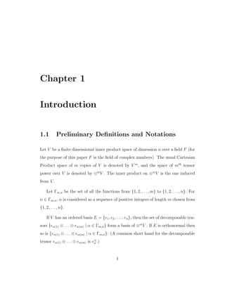
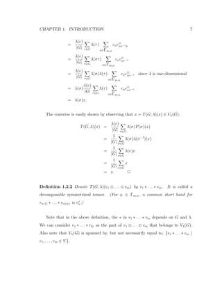
Proposition 1.1.2 With respect to the induced inner product, T(G, λ) is an or-
thogonal projection.
Proof: We use the following result from group representation theory: Let λ and
χ be irreducible characters of the finite group G afforded by representations A and
B of G respectively. Then for any π ∈ G,
σ∈G
λ(σ−1
)χ(σπ) =
|G|λ(π)/λ(e) if A ≡ B,
0 otherwise
(1.2)
(see [37], page 11).
We have:
T(G, λ)T(G, λ) =
λ(e)2
|G|2
σ∈G
λ(σ)P(σ)
τ∈G
λ(τ)P(τ)
=
λ(e)2
|G|2
σ,τ∈G
λ(σ)λ(τ)P(στ)
=
λ(e)2
|G|2
π∈G σ∈G
λ(σ)λ(σ−1
π) P(π) by writing π = στ
=
λ(e)
|G| π∈G
λ(π)P(π) by (1.2)
= T(G, λ).
Thus T(G, λ) is a projection.
By straight-forward calculations, it is easily shown that
λ(e)
|G| σ∈G
λ(σ)P(σ)∗
(where λ(σ) denotes the complex conjugate of λ(σ)) has all the properties of
T(G, λ)∗
. By the uniqueness of adjoints and the fact that P(σ)∗
= P(σ−1
), we
have
T(G, λ)∗
=
λ(e)
|G| σ∈G
λ(σ)P(σ)∗
=
λ(e)
|G| σ∈G
λ(σ−1
)P(σ−1
) = T(G, λ). 2](https://image.slidesharecdn.com/9030f5f3-c79f-4e09-99b4-6f509ca53797-160820195713/85/MMath-11-320.jpg)
![CHAPTER 1. INTRODUCTION 5
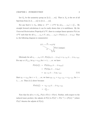
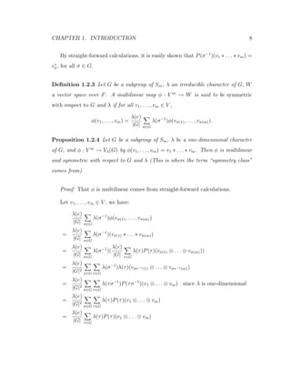
Theorem 1.1.3 Let I(G) denote the set of all irreducible characters of G, where
G is a subgroup of Sm. If λ, χ ∈ I(G) and λ = χ, then T(G, λ) ◦ T(G, χ) = 0.
Moreover,
λ∈I(G)
T(G, λ) is the identity map on ⊗m
V .
Proof: Using (1.2), we have:
T(G, λ)T(G, χ) =
λ(e)χ(e)
|G|2
π∈G σ∈G
λ(σ)χ(σ−1
π) P(π)
= 0.
To show that
λ∈I(G)
T(G, λ) = I⊗mV , we use the following result from group
representation theory:
Let σ ∈ G, where G is any finite group. Then
χ∈I(G)
χ(e)χ(σ) =
|G| if σ = e,
0 otherwise
(1.3)
(see [37], page 17).
Using (1.3), we get:
λ∈I(G)
T(G, λ) =
λ∈I(G)
(
λ(e)
|G| σ∈G
λ(σ)P(σ))
=
1
|G| λ∈I(G)
λ(e)
σ∈G
λ(σ)P(σ)
=
1
|G| σ∈G
(
λ∈I(G)
λ(e)λ(σ))P(σ)
= P(e)
= I⊗mV . 2
Definition 1.1.4 Vλ(G) is a subspace of ⊗m
V (since T(G, λ) is linear), and is
called the symmetry class of tensors associated with G and λ.](https://image.slidesharecdn.com/9030f5f3-c79f-4e09-99b4-6f509ca53797-160820195713/85/MMath-12-320.jpg)
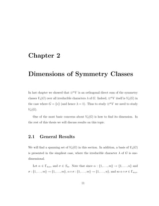
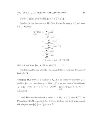
![CHAPTER 2. DIMENSIONS OF SYMMETRY CLASSES 18
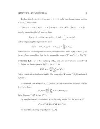
Conversely, α ∈ Ω means
τ∈Gα
λ(τ) = 0 which, by the discussion after lemma
2.1.3, is equivalent to e∗
α = 0, i.e., e∗
αe = 0. Thus {e∗
ασ | σ ∈ G} = {0}, giving
sα = 0.
2. This is the last part in the proof of theorem 2.1.7.
3. By theorem 2.1.6, Vλ(G) =
α∈
span{e∗
ασ | σ ∈ G}, the sum being direct.
This immediately gives us the result. 2
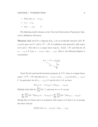
In [9], R. Freese gave the following general formula for sα:
Theorem 2.2.3 (Freese) For α ∈ Γm,n, sα = λ(e)(λ, 1)Gα , where
(λ, 1)Gα =
1
|Gα| σ∈Gα
λ(σ).
To prove Freese’s theorem, we first prove the following well known result in
linear algebra:
Lemma 2.2.4 The rank of an idempotent linear operator on a vector space is its
trace.
Proof: Let L : V → V be an idempotent linear operator on the n-dimensional
space V . Let R and N denote the image and kernel of L respectively.
It is easy to see that v ∈ R if and only if v = L(v), for if v = L(u) for some
u ∈ V , then since L is idempotent, L(v) = L2
(u) = L(u) = v; and if v = L(v), then
(obviously) v ∈ R.
Thus we have R ∩ N = {0}. Further, since every vector v ∈ V can be written
as v = L(v) + (v − L(v)), and v − L(v) ∈ N, we conclude that V is a direct sum of
R and N.](https://image.slidesharecdn.com/9030f5f3-c79f-4e09-99b4-6f509ca53797-160820195713/85/MMath-25-320.jpg)
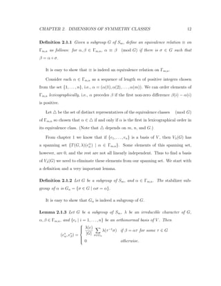
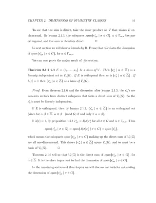
![CHAPTER 2. DIMENSIONS OF SYMMETRY CLASSES 22
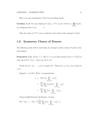
2.3 Using Disjoint Cycle Decomposition of Sm
In [26], M. Marcus gave a formula for the rank of the linear operator T(G, λ), that
is, the dimension of Vλ(G). The method uses the disjoint cycle decomposition of
elements of Sm. To prove that result we first prove the following lemma.
Lemma 2.3.1 Let σ ∈ Sm and let c(σ) denote the number of cycles in the dis-
joint cycle decomposition of σ, including cycles of length one. Then for the linear
operation P(σ) on ⊗m
V , trace(P(σ)) = nc(σ)
.
Proof: Let {e1, . . . , en} be a basis of V , {f1, . . . , fn} be the basis of V ∗
dual to
{e1, . . . , en}, i.e.,
fi(ej) =
1 if i = j
0 otherwise
extended linearly to all of V ∗
.
Let E = {e⊗
α | α ∈ Γm,n} be the corresponding (ordered) basis of ⊗m
V . For
each β ∈ Γm,n, define a linear functional hβ : ⊗m
V → F by extending
hβ(eα(1) ⊗ . . . ⊗ eα(m)) = fβ(1)(eα(1)) . . . fβ(m)(eα(m)) =
m
i=1
fβ(i)(eα(i))
To all of ⊗m
V . We have
hβ(e⊗
α ) =
1 if α = β
0 otherwise.
This means that {hβ | β ∈ Γm,n} is the basis of (⊗m
V )∗
dual to E.
The elements on the main diagonal of the matrix representing P(σ) with respect
to E are the numbers
hα(P(σ)(e⊗
α )) = hα(e⊗
ασ−1 )](https://image.slidesharecdn.com/9030f5f3-c79f-4e09-99b4-6f509ca53797-160820195713/85/MMath-29-320.jpg)
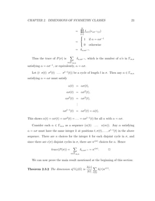
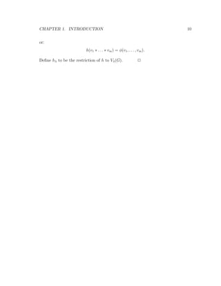
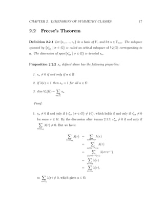
![CHAPTER 2. DIMENSIONS OF SYMMETRY CLASSES 24
Proof: By proposition 1.1.2 T(G, λ) is idempotent. We have:
dim Vλ(G) = rank(T(G, λ))
= trace(T(G, λ)) by lemma 2.2.4
= trace(
λ(e)
|G| τ∈G
λ(τ)P(τ))
=
λ(e)
|G| τ∈G
λ(τ)trace(P(τ))
=
λ(e)
|G| τ∈G
nc(τ)
by lemma 2.3.1. 2
2.4 Subspaces of the Orbital Subspaces
In [46] B. Y. Wang and M. P. Gong described methods to construct subspaces of
the orbital subspaces span{e∗
ασ | σ ∈ G}, α ∈ , and calculate their dimensions.
Some of their results are summarized in this section.
As before, let G be a subgroup of Sm with identity element e, and let {e1, . . . , en}
be a fixed orthonormal basis of V , so that {e⊗
α | α ∈ Γm,n} is an orthonormal basis
of ⊗m
V . Let A be an irreducible representation of G which affords the irreducible
character λ. For each σ ∈ G and i, j ∈ {1, . . . , λ(e)}, let aij(σ) denote the (i, j)th
element of the matrix A(σ) with respect to the basis {e1, . . . , en}.
Define the operators Tij on ⊗m
V by
Tij =
λ(e)
|G| σ∈G
aij(σ)P(σ)
for each i, j = 1, . . . , λ(e).
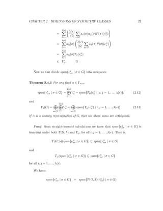
By straight-forward calculations we see that
T(G, λ) =
λ(e)
i=1
Tii.](https://image.slidesharecdn.com/9030f5f3-c79f-4e09-99b4-6f509ca53797-160820195713/85/MMath-31-320.jpg)
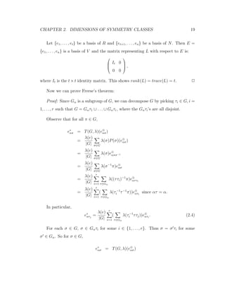
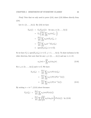
![CHAPTER 2. DIMENSIONS OF SYMMETRY CLASSES 25
We further have the following identities:
T2
ii = Tii (2.5)
and
TijTkl =
Til if j = k,
0 otherwise
(2.6)
for all i, j, k, l ∈ {1, . . . , λ(e)} (see [37], page V-8).
If A is a unitary representation (that is, A(σ)A(σ)∗
= A(σ)∗
A(σ) = I, or that
A(σ) is a unitary matrix, for every σ ∈ G), then
T∗
ij = Tji (2.7)
for all i, j ∈ {1, . . . , λ(e)}.
Let V ij
A (G) = Tij(⊗m
V ). We have the following theorem:
Theorem 2.4.1 The symmetry class of tensors, Vλ(G), is equal to
λ(e)
i=1
V ii
A (G), a
direct sum, and dim V ii
A (G) =
dim Vλ(G)
λ(e)
. If A is a unitary representation of G,
then the sum is orthogonal. 2
(see [37], page V-8).
Let α ∈ Γm,n. To divide span{e∗
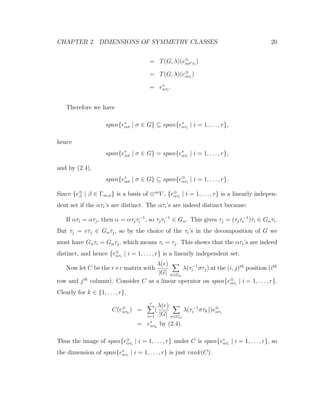
ασ | σ ∈ G} into subspaces, we first introduce a
lemma:
Lemma 2.4.2 Let V i
α = span{Ti1(e⊗
α ), . . . , Tiλ(e)(e⊗
α )}, for i = 1, . . . , λ(e). Then
V i
α = span{Tij(e⊗
ασ) | σ ∈ G, j = 1, . . . , λ(e)}, for i = 1, . . . , λ(e) (2.8)
and
V i
ατ = V i
α, for all τ ∈ G and i = 1, . . . , λ(e). (2.9)](https://image.slidesharecdn.com/9030f5f3-c79f-4e09-99b4-6f509ca53797-160820195713/85/MMath-32-320.jpg)
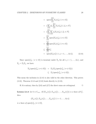
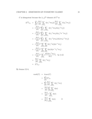
![CHAPTER 2. DIMENSIONS OF SYMMETRY CLASSES 30
Thus Ei also spans V i
α. Hence Ei is a basis of V i
α. 2
The above lemma shows that if we know how to calculate dim V i
α, we can then
easily find the dimension of span{e∗
ασ | σ ∈ G}. The following theorem does exactly
that:
Theorem 2.4.5 dim V i
α = (λ, 1)Gα , where
(λ, 1)Gα =
1
|Gα| σ∈Gα
λ(σ),
for all i = 1, . . . , λ(e).
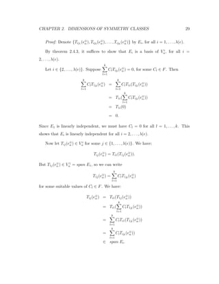
Proof: By lemma 2.4.4 all subspaces V i
α have the same dimensions. Using this
result and theorem 2.4.3, we have:
dim V i
α =
dim span{e∗
ασ | σ ∈ G}
λ(e)
for each i = 1, . . . , λ(e). Freese’s theorem gives
dim span{e∗
ασ | σ ∈ G} = λ(e)(λ, 1)Gα
which leads directly to our result. 2
If the irreducible representation A of G is unitary, we can then construct or-
thonormal bases of all the orbital subspaces of Vλ(G). Before we do that, first we
introduce a couple of notation:
If A is a p × q matrix and i1, . . . , ik, j1, . . . , jl are positive integers with i1 <
. . . < ik ≤ p and j1 < . . . < jl ≤ q, let A[i1, . . . , ik | j1, . . . , jl] denote the k × l
matrix whose element at row s and column t is the element at row is and column
jt of the matrix A.](https://image.slidesharecdn.com/9030f5f3-c79f-4e09-99b4-6f509ca53797-160820195713/85/MMath-37-320.jpg)
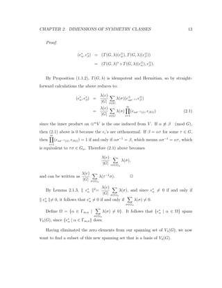
![CHAPTER 2. DIMENSIONS OF SYMMETRY CLASSES 31
For α ∈ Γm,n, let
dj =
λ(e)
|G| σ∈Gα
ajj(σ)
for j = 1, . . . , λ(e). We have the following:
Theorem 2.4.6 Let A be an irreducible and unitary representation of G. Let α ∈
Γm,n and k = (λ, 1)Gα . If there exist j1, . . . , jk such that
σ∈Gα
A(σ)[j1, . . . , jk | j1, . . . , jk]
is a diagonal matrix, and djl
= 0 for all l = 1, . . . , k, then
E =
1
djl
Tijl
(e⊗
α ) | i = 1, . . . , λ(e), l = 1, . . . , k
is an orthonormal basis of the orbital subspace span{e∗
ασ | σ ∈ G}.
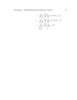
Proof: By the proof of theorem 2.4.5 above, we know that E contains the
right number of elements. So all we need to do is to show that elements in E are
orthonormal.
Using the identities (2.6) and (2.7), we obtain
1
djt
Tijt (e⊗
α ),
1
djs
Trjs (e⊗
α )
=
1
djt djs
(Tijt (e⊗
α ), Trjs (e⊗
α ))
=
1
djt djs
(TjsrTijt (e⊗
α ), e⊗
α )
=
1
djt djs
δir(Tjsjt (e⊗
α ), e⊗
α )
=
δir
djt djs
λ(e)
|G| σ∈G
ajsjt (σ)P(σ)(e⊗
α ), e⊗
α
=
δir
djt djs
λ(e)
|G| σ∈G
ajsjt (σ)(e⊗
ασ−1 ), e⊗
α](https://image.slidesharecdn.com/9030f5f3-c79f-4e09-99b4-6f509ca53797-160820195713/85/MMath-38-320.jpg)
![Chapter 3
Some Special Results
3.1 General Results on Cyclic Groups
In [13] R. Holmes and T. Tam discussed some results regarding cyclic groups. Their
results are presented here.
Let r ∈ Sm be an m-cycle (e.g., the cycle (1 2 . . . m)). Then the subgroup
of Sm generated by r is the cyclic group Cm. The elements of Cm are rk
, for
k = 0, . . . , m − 1.
For convenience in notation, in the following discussions we assume that r is
the m-cycle (1 2 . . . m). The result is the same for other m-cycles.
We the have the following result:
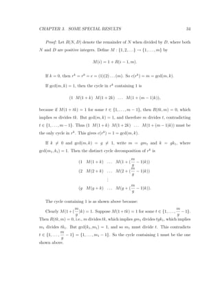
Proposition 3.1.1 Using the above notation, for any rk
∈ Cm, c(rk
) = gcd(m, k).
(where c(g) is the number of cycles in the disjoint cycle decomposition of g, as
defined in lemma 2.3.1)
33](https://image.slidesharecdn.com/9030f5f3-c79f-4e09-99b4-6f509ca53797-160820195713/85/MMath-40-320.jpg)
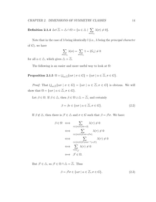
![CHAPTER 3. SOME SPECIAL RESULTS 35
By the same reasoning, the cycles containing 2, 3, . . . , g are also as shown above.
Thus c(rk
) = g = gcd(m, k). 2
For π ∈ Sm, define bi(π) to be the number of cycles of length i in the disjoint
cycle decomposition of π. Clearly for any i > m, bi(π) = 0, and the function c(π)
in the proposition above is precisely
m
i=1
bi(π)
and is called the type of π.
Let r ∈ Sm be an m−cycle. Then the subgroup of Sm generated by r is the
cyclic group Cm. The elements of Cm are rk
, for k = 0, . . . , m − 1.
By proposition 3.1.1, c(rk
) = gcd(m, k) for k = 0, . . . , m − 1, so c(rk
) divides
m. On the other hand, for any k that divides m, k = gcd(m, k) = c(rk
). Thus the
types of elements of G constitute exactly the set of divisors of m, i.e.,
{c(σ) | σ ∈ G} = {d | d divides m}.
Since Cm is Abelian, from group representation theory we know that all of its
irreducible representations are of degree one. Thus for any irreducible character λ
of Cm, λ(Cm) is a group of complex roots of unity. Therefore the m irreducible
characters of Cm are:
λl(rk
) = e2πilk/m
, for l = 0, . . . , m − 1 (3.1)
(see [45], page 35). Since each λl is of degree one, by theorem 2.1.7, {e∗
α | α ∈ }
is a basis of Vλl
(Cm), so dimVλl
(Cm) = | |.
Another way to find the dimension of Vλl
(Cm) is to use the following formula
given by R. Holmes and T. Tam in [13]:](https://image.slidesharecdn.com/9030f5f3-c79f-4e09-99b4-6f509ca53797-160820195713/85/MMath-42-320.jpg)
![CHAPTER 3. SOME SPECIAL RESULTS 36
Theorem 3.1.2 dim Vλl
(Cm) =
1
m
m−1
k=1
e2πilk/m
ngcd(m,k)
, for l = 0, . . . , m − 1.
Proof: By theorem 2.3.2,
dim Vλl
(Cm) =
λl(e)
|Cm| σ∈Cm
λl(σ)nc(σ)
=
1
m
m−1
k=0
λl(rk
)nc(rk)
=
1
m
m−1
k=0
e2πilk/m
ngcd(m,k)
by (3.1) and proposition 3.1.1. 2
3.2 Simplified Formulas for Cyclic Groups
Although the results presented in the last chapter and the previous section are of
theoretical importance, they are difficult to use to actually calculate the dimen-
sion of some symmetry class. In [5], L. J. Cummings gave three formulas that
greatly simplify the necessary calculations in some special cases. Those results are
presented in this section.
Definition 3.2.1 For each positive integer p, let φ(p) denote the number of integers
in {1, 2, . . . , p} that are coprime with p. The function φ is called the Euler Totient
Function.
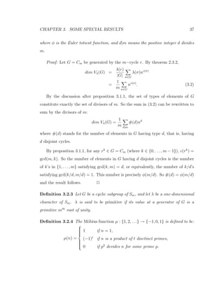
Theorem 3.2.2 Let G = Cm be a subgroup of Sm generated by an m−cycle, and
let λ be the character identically 1. Then
dimVλ(G) =
1
m d|m
φ(m/d)nd
,](https://image.slidesharecdn.com/9030f5f3-c79f-4e09-99b4-6f509ca53797-160820195713/85/MMath-43-320.jpg)
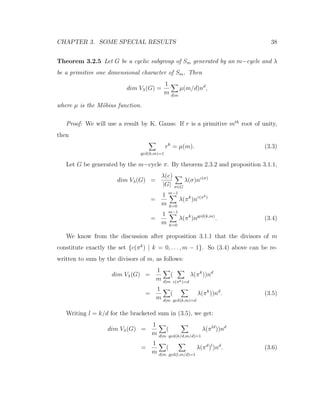
![CHAPTER 3. SOME SPECIAL RESULTS 40
Since the πi’s are disjoint and G = π1, . . . , πk , we must have
{π
f(1)
1 . . . π
f(k)
k | f ∈ F} = G,
and
rf =
k
i=1
c(π
f(i)
i ) = c(π
f(1)
1 . . . π
f(k)
k ).
So equation (3.8) above becomes
k
i=1
dim Vλ( πi ) =
1
m g∈G
nc(g)
λ(g)
= dim Vλ(G). 2
3.3 Dihedral Groups
In [13] R. Holmes and T. Tam analyzed the dihedral subgroup Dm of Sm (m ≥ 3).
Consider the elements r, s ∈ Sm with
r = (1 2 . . . m)
and
s =
(2 m)(3 m − 1) . . . (
m
2
m
2
+ 2) if m is even
(2 m)(3 m − 1) . . . (
m + 1
2
m + 3
2
) if m is odd.
The subgroup of Sm generated by r and s is Dm, the dihedral group of degree m.
Clearly, it contains the cyclic subgroup Cm (since Cm = r ). By straight-forward
calculations we see that r, s satisfy
rm
= s2
= e and srs = r−1
. (3.9)
Further,
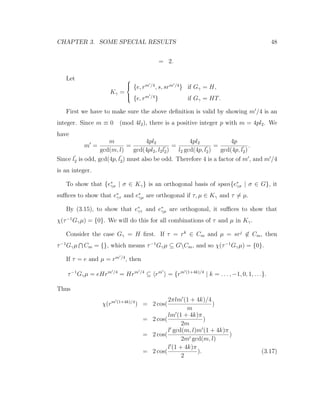
Dm = {rk
, srk
| k = 0, . . . , m − 1} (3.10)](https://image.slidesharecdn.com/9030f5f3-c79f-4e09-99b4-6f509ca53797-160820195713/85/MMath-47-320.jpg)
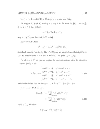
![CHAPTER 3. SOME SPECIAL RESULTS 41
(see [14], pages 50-51).
For each integer l with 0 < l < m/2, Dm has an irreducible character χl of
degree 2 which is induced from the irreducible character λl of Cm in (3.1):
χl(rk
) = 2 cos(
2πlk
m
)
χl(srk
) = 0 (3.11)
for k = 0, . . . , m − 1. All other irreducible characters of Dm are of degree 1 (see
[45], page 37).
Also note that for any integer k, by (3.9), we have:
srk
= sr(ss)rk−1
= (srs)srk−1
= r−1
srk−1
...
= r−k
s. (3.12)
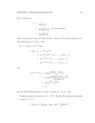
Theorem 3.3.1 Let {e1, . . . , en} be an orthonormal basis of V with n ≥ 2, G =
r, s = Dm with m ≥ 3, and χ = χl for some 0 < l < m/2. There is a subset S of
Γm,n for which
{e∗
γ | γ ∈ S}
is an orthogonal basis of Vχ(G), if and only if
m ≡ 0 (mod 4l2)
where l = l2l2 with l2 being the largest power of 2 dividing l, and l2 being odd.
Proof: First suppose Vχ(G) has an orthogonal basis {e∗
γ | γ ∈ S} for some subset
S of Γm,n.](https://image.slidesharecdn.com/9030f5f3-c79f-4e09-99b4-6f509ca53797-160820195713/85/MMath-48-320.jpg)
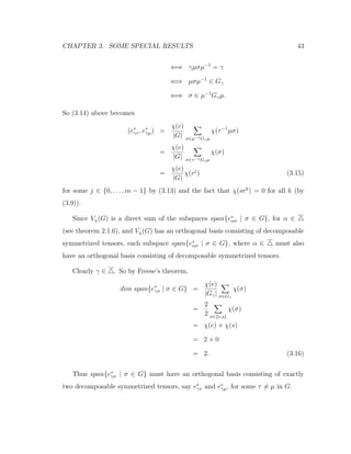
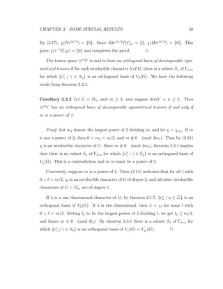
![CHAPTER 3. SOME SPECIAL RESULTS 44
If χ = 0 on Cm, then by (3.15) (e∗
γτ , e∗
γµ) = 0 and so e∗
γτ and e∗
γµ can not be
orthogonal to each other. This contradiction shows that χ must vanish for some
element in Cm.
Consequently, we must have
χ(rk
) = 2 cos(
2πlk
m
) = 0
for some k. That is,
2πlk
m
=
(2h + 1)π
2
for some integer h. This means 4lk = (2h + 1)m, or 4l2l2k = (2h + 1)m, where
l2l2 = l and l2 is the largest power of 2 dividing l. Since (2h + 1) is odd, 4l2 must
divide m. Hence m ≡ 0 (mod 4l2).
Conversely, suppose m ≡ 0 (mod 4l2). Let γ ∈ , and let H = Gγ ∩ Cm. We
can easily check that H is a subgroup of Cm.
Recall that χ = χl is the induced character λG
where λ = λl (see (3.11)).
Denote the restrictions to H of χ and λ by χH and λH respectively. Using Mackey’s
subgroup theorem (see [45], page 58) we get
χH = (λG
)H = λH + (λH)s
where (λH)s
is the character of H defined by:
(λH)s
(rk
) = λH(s−1
rk
s)
= λH(s−1
sr−k
) by (3.12)
= λH(r−k
)
= λH(rk
)−1](https://image.slidesharecdn.com/9030f5f3-c79f-4e09-99b4-6f509ca53797-160820195713/85/MMath-51-320.jpg)
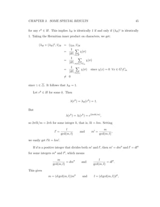
![CHAPTER 3. SOME SPECIAL RESULTS 46
which implies (d gcd(m, l)) is a common factor of m and l. Thus d must be 1, and
so m and l are coprime.
Since l k = hm , we have k = (hm )/l = m (h/l ). If (h/l ) is not an integer,
then there is a prime factor p of l which divides m but does not divide h. This
cannot happen because m and l are coprime. So (h/l ) must be an integer.
Since k = m (h/l ), and (h/l ) is an integer, we have rk
∈ rm
. But rk
is
arbitrary in H, so we conclude that H is a subgroup of rm
.
Suppose Gγ = H. Then Gγ contains some t ∈ GγCm ⊆ GCm, which means
t must be in the form srk
for some integer k. By (3.12) we have t2
= e, and so
T = {t, e} is a subgroup of Gγ.
For any g ∈ Gγ, if g = rj
for some j, then clearly gH = Hg. If g = srj
for some
j, then for any h = rk
∈ H, by (3.9) and (3.12) we have:
gh = (ghg−1
)g = (srj
rk
(srj
)−1
)g = (srj+k
r−j
s−1
)g = (srk
s−1
)g = r−k
g = h−1
g,
so again we have gH = Hg. This indicates that H is a normal subgroup of Gγ,
and hence HT is a subgroup of Gγ. Since T = {t, e}, we have |HT| = 2|H|.
For any g ∈ G, either g = rk
or g = srk
for some integer k. If g = rk
then
g = rk
e ∈ CmGγ. If g = srk
, let t = srj
∈ Gγ for some integer j (t = rj
for any j
because t ∈ Cm). By (3.9) and (3.12) we have:
g = srk
= srk−j
rj
= srk−j
(ss)rj
= (srk−j
s)(srj
) = (rj−k
ss)t = rj−k
t ∈ CmGγ.
So G ⊆ CmGγ, which gives G = CmGγ.
By the Second Group Isomorphism Theorem (see [14], page 44),
Gγ/H = Gγ/(Cm ∩ Gγ) ∼= CmGγ/Cm = G/Cm.](https://image.slidesharecdn.com/9030f5f3-c79f-4e09-99b4-6f509ca53797-160820195713/85/MMath-53-320.jpg)
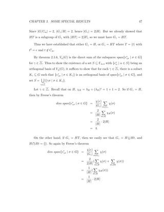
![CHAPTER 3. SOME SPECIAL RESULTS 51
3.4 Linear Symmetry Classes
In [7] L. J. Cummings and R. W. Robinson used P´olya’s counting theorem to
calculate the dimension of V1(G), the linear symmetry class associated with the
principal character (i.e., identically 1). The results from their work is summarized
in this section.
We first introduce some notations and P´olya’s counting theorem.
Let G be a subgroup of Sm acting on Γm,n by
g · α = α ◦ g−1
for all g ∈ G and α ∈ Γm,n.
For each g ∈ G, denote the number of cycles of length i in the cyclic decompo-
sition of g by bi(g) (as defined after proposition 3.1.1).
The cycle type of g ∈ G is the monomial
Z(g) = Z(g; a1, . . . , am) =
m
k=1
a
bk(g)
k
in the variables a1, . . . , am. The cycle index of G is the polynomial
Z(G) = Z(G; a1, . . . , am) =
1
|G| g∈G
Z(g).
If A is a commutative ring and w : {1, . . . , n} → A, then the elements w(i) are
called weights. The weight of a function α ∈ Γm,n is
W(α) =
m
i=1
w(α(i)).
It is easy to show that if two functions α, β ∈ Γm,n are in the same orbit of Γm,n
under the action of G then W(α) = W(β).](https://image.slidesharecdn.com/9030f5f3-c79f-4e09-99b4-6f509ca53797-160820195713/85/MMath-58-320.jpg)
![CHAPTER 3. SOME SPECIAL RESULTS 52
Note that the orbits of Γm,n under the action of G are precisely the equivalence
classes of Γm,n defined in definition 2.1.1, and is a traversal of these equivalence
classes or orbits.
If W(α) is the weight of a representative of an orbit, then the result of summing
the weights of representatives over all orbits (e.g., summing over ,
α∈
W(α)) is
called the pattern inventory of the equivalence classes. This pattern inventory can
be calculated using P´olya’s Counting Theorem:
Theorem 3.4.1 (P´olya’s Counting Theorem)
α∈
W(α) = Z(G;
n
i=1
w(i), . . . ,
n
i=1
(w(i))m
)
=
1
|G| g∈G
(
m
k=1
(
n
i=1
(w(i))k
)bk(g)
). 2
(For a complete proof of P´olya’s Counting Theorem, see [23], chapter 5.)
Corollary 3.4.2 If G is a subgroup of Sm then the number of G-orbits in Γm,n
(i.e., | |) is Z(G; n, . . . , n).
Proof: Let w : {1, . . . , n} → {1}. Then for all α ∈ Γm,n,
W(α) =
m
i=1
w(α(i)) = 1.
By P´olya’s counting theorem we have
| | =
α∈
1
=
α∈
W(α)
= Z(G;
n
i=1
w(i), . . . ,
n
i=1
(w(i))m
)
= Z(G; n, . . . , n). 2](https://image.slidesharecdn.com/9030f5f3-c79f-4e09-99b4-6f509ca53797-160820195713/85/MMath-59-320.jpg)
![CHAPTER 3. SOME SPECIAL RESULTS 53
Theorem 3.4.3 If λ is the principal character of G (i.e., identically 1), then
dim Vλ(G) =
1
|G| g∈G
Z(g; n, . . . , n).
Proof: Since λ is identically 1, by the remark after definition 2.1.4, we have
= . By theorem 2.1.7 and corollary 3.4.2,
dim Vλ(G) = | | = | | = Z(G; n, . . . , n),
which by definition is
1
|G| g∈G
Z(g) =
1
|G| g∈G
Z(g; n, . . . , n). 2
3.5 Counting Restricted Orbits
In [7] section 3 L. J. Cummings and R. W. Robinson studied the action of a subgroup
of Sm acting on a finite set X equipped with a linear (one-dimensional) character,
λ. They developed a formula for counting special orbits of X under the action of
G, and applied that formula to calculate dim Vλ(G) when X = Γm,n. Their results
are presented in this section.
Let G be a subgroup of Sm acting on a finite set X (later the results obtained
here will be applied to X = Γm,n, with g(α) = g · α = α ◦ g−1
for all g ∈ G and
α ∈ Γm,n). For α ∈ X, let Gα = {g ∈ G | g · α = α} be the stabilizer subgroup
of α. For any g ∈ G, let F(g) denote the number of elements in X left fixed by g.
Burnside’s lemma (see [10], pages 134-135) states that the number of orbits of X
under the action of G is
1
|G| g∈G
F(g).](https://image.slidesharecdn.com/9030f5f3-c79f-4e09-99b4-6f509ca53797-160820195713/85/MMath-60-320.jpg)
![CHAPTER 3. SOME SPECIAL RESULTS 54
For any positive integer k, denote the group of complex kth
roots of unity by
Ck. If λ is a linear character of G, then λ(G) = Cc for some c. For each α ∈ X,
let σ(α) be determined by λ(Gα) = Cσ(α). If α and β are in the same G-orbit (i.e.,
α = g · β for some g ∈ G) then we can easily show that Gα and Gβ are conjugate
(i.e., Gα = gGβg−1
for some g ∈ G), so λ(Gα) = λ(Gβ), and hence σ(α) = σ(β).
For any g ∈ G, denote the order of λ(g) by λ(g)◦
. A new character λk of G can be
obtained by defining
λk(g) = (λ(g))k
for each g ∈ G. We have the following theorem:
Theorem 3.5.1 With the above set-up, suppose λ(G) = Cc with k|c. Then the
number of G-orbits consisting of α ∈ X with σ(α) = k is
ak =
1
|G| g∈G
F(g)(
v|k
µ(λv(g)◦
)
φ(λv(g)◦
)
)µ(k/v),
where µ is the M¨obius function, and φ is the Euler totient function. 2
(See [7], pages 1315-1317 for a complete proof.)
Now let G act on Γm,n by g(α) = g · α = α ◦ g−1
for all g ∈ G and α ∈ Γm,n.
The basic result of L. J. Cummings and R. W. Robinson (see [7]) implies
dim Vλ(G) = a1. (3.18)
By the second half of the proof of lemma 2.3.1, F(g) = nc(g)
, where c(g) is the
number of cycles in the disjoint cycle decomposition of g. Thus using (3.18) and
straight-forward calculations we obtain the following result:
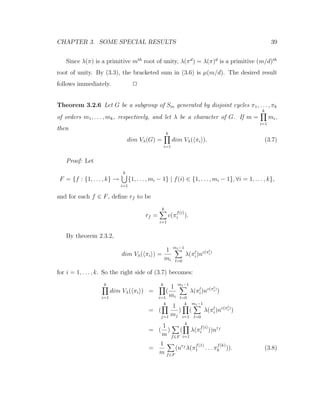
Theorem 3.5.2 If G is a subgroup of Sm and λ is a one-dimensional character of
G, then
dim Vλ(G) =
1
|G| g∈G
µ(λ(g)◦
)
φ(λ(g)◦
)
nc(g)
. 2](https://image.slidesharecdn.com/9030f5f3-c79f-4e09-99b4-6f509ca53797-160820195713/85/MMath-61-320.jpg)
![Bibliography
[1] G. H. Chan. On the Triviality of a Symmetry Class of Tensors, Linear and
Multilinear Algebra, Vol. 6, No. 1, 1978/79, pp. 73-82.
[2] G. H. Chan. (k)-Characters and the Triviality of Symmetry Classes II, Nanta
Mathematica, Vol. 12, No. 1, 1979, pp. 7-15.
[3] G. H. Chan and M. H. Lim. Nonzero Symmetry Classes of Smallest Dimension,
Canadian Journal of Mathematics, Vol. 32, No. 4, 1980, pp. 957-968.
[4] L. J. Cummings. Decomposable Symmetric Tensors, Pacific Journal of Math-
ematics, Vol. 35, No. 1, 1970, pp. 65-77.
[5] L. J. Cummings. Cyclic Symmetry Classes, Journal of Algebra, Vol. 40, No. 2,
June 1976, pp. 401-404.
[6] L. J. Cummings. Transformations of Symmetric Tensors. Pacific Journal of
Mathematics, Vol. 42, No. 3, 1972, pp. 603-613.
[7] L. J. Cummings and R. W. Robinson. Linear Symmetry Classes, Canadian
Journal of Mathematics, Vol. XXVIII, No. 6, 1976, pp. 1311-1318.
[8] Charles W. Curtis and Irving Reiner. Representation Theory of Finite Groups
and Associative Algebras. John Wiley & Sons, New York, 1962.
55](https://image.slidesharecdn.com/9030f5f3-c79f-4e09-99b4-6f509ca53797-160820195713/85/MMath-62-320.jpg)
![BIBLIOGRAPHY 56
[9] R. Freese. Inequalities for Generalized Matrix Functions Based on Arbitrary
Characters, Linear Algebra Appl. 7, (1973), pp. 337-345.
[10] William J. Gilbert. Modern Algebra with Applications. John Wiley & Sons,
U.S.A., 1976.
[11] J. Hillel. Algebras of Symmetry Classes of Tensors and Their Underlying Per-
mutation Groups, Journal of Algebra, Vol. 23, 1972, pp. 215-227.
[12] J. Hillel. Dimensionality of Algebras of Symmetry Classes of Tensors, Linear
and Multilinear Algebra, Vol. 4, No. 1, 1976, pp. 41-44.
[13] Randal R. Holmes and Tin-Yau Tam. Symmetry Classes of Tensors Associated
with Certain Groups, Linear and Multilinear Algebra, Vol. 32, 1992, pp. 21-31.
[14] Thomas W. Hungerford. Algebra. Springer-Verlag, New York, 1974.
[15] Ohoe Kim, John Chollet, Ralf Brown, and David Rauschenberg. Orthonormal
Bases of Symmetry Classes with Computer-Generated Examples, Linear and
Multilinear Algebra, Vol. 21, No. 1, 1987, pp. 91-106.
[16] M. H. Lim. A Note on Maximal Decomposable Subspaces of Symmetry Classes,
Tamkang Journal of Mathematics, Vol. 5, 1974, pp. 241-246.
[17] M. H. Lim. Some Remarks Concerning Permutations on Symmetry Classes,
Kyungpook Mathematical Journal, Vol. 14, 1974, pp. 261-266.
[18] M. H. Lim. Regular Symmetry Classes of Tensors, Nanta, Vol. 8, No. 2, 1975,
pp. 42-46.
[19] M. H. Lim. Linear Transformations on Symmetry Classes of Tensors, Linear
and Multilinear Algebra, Vol. 3, No. 4, 1976, pp. 267-280.](https://image.slidesharecdn.com/9030f5f3-c79f-4e09-99b4-6f509ca53797-160820195713/85/MMath-63-320.jpg)
![BIBLIOGRAPHY 57
[20] M. H. Lim. A Uniqueness Theorem in Symmetry Classes, Linear and Multi-
linear Algebra, Vol. 4, No. 2, 1976/77, pp. 85-88.
[21] M. H. Lim. Rank k Vectors in Symmetry Classes of Tensors, Canadian Math-
ematics Bulletin, Vol. 19, No. 1, 1976, pp. 67-76.
[22] M. H. Lim. Linear Mappings on Symmetry Classes of Tensors, Linear and
Multilinear Algebra, Vol. 12, No. 2, 1982/83, pp. 109-123.
[23] C. L. Liu. Introduction to Combinatorial Mathematics. McGraw-Hill Book
Company, U.S.A., 1968.
[24] Jerry Malzan. On Symmetry Classes of Tensors, Mathematical Reports of the
Academy of Sciences, the Royal Society of Canada, Vol. 3, No. 3, 1981, pp.
165-169.
[25] Marvin Marcus. Lengths of Tensors. Academic Press, New York, 1967.
[26] Marvin Marcus. Finite Dimensional Multilinear Algebra, Part I. Marcel
Dekker, Inc., New York, 1973.
[27] Marvin Marcus. Finite Dimensional Multilinear Algebra, Part II. Marcel
Dekker, Inc., New York, 1975.
[28] Marvin Marcus and John Chollet. Decomposable Symmetrized Tensors, Linear
and Multilinear Algebra, Vol. 6, No. 4, 1978, pp. 317-326.
[29] Marvin Marcus and John Chollet. The Index of a Symmetry Class of Tensors,
Linear and Multilinear Algebra, Vol. 11, No. 3, 1982, pp. 277-281.
[30] Marvin Marcus and John Chollet. On the Equality of Decomposable Sym-
metrized Tensors, Linear and Multilinear Algebra, Vol. 13, No. 3, 1983, pp.
253-266.](https://image.slidesharecdn.com/9030f5f3-c79f-4e09-99b4-6f509ca53797-160820195713/85/MMath-64-320.jpg)
![BIBLIOGRAPHY 58
[31] Marvin Marcus and John Chollet. Construction of Orthonormal Bases in
Higher Symmetry Classes of Tensors, Linear and Multilinear Algebra, Vol.
19, No. 2, 1986, pp. 133-140.
[32] Marvin Marcus and John Chollet. Lower Bounds for the Norms of Decom-
posable Symmetrized Tensors, Linear and Multilinear Algebra, Vol. 25, No. 4,
1989, pp. 269-274.
[33] Marvin Marcus and William R. Gordon. The Structure of Bases in Tensor
Spaces, American Journal of Mathematics, Vol. 92, 1970, pp. 623-640.
[34] Marvin Marcus and B. N. Moyls. Transformations on Tensor Product Spaces,
Pacific Journal of Mathematics, Vol. 9, 1959, pp. 1215-1221.
[35] Marvin Marcus and Henryk Minc. Permutations on Symmetry Classes, Journal
of Algebra, Vol. 5, 1967, pp. 59-71.
[36] Marvin Marcus and Henryk Minc. Generalized Matrix Functions, Transactions
of the American Mathematical Society, Vol. 116, 1965, pp. 316-329.
[37] Russell Merris. Multilinear Algebra. California State University, Hayward
[38] Russell Merris. The Structure of Higher Degree Symmetry Classes of Tensors,
Mathematical Sciences, Section B, Journal of Research of the National Bureau
of standards, 80B, No. 2, 1976, pp. 259-264.
[39] Russell Merris. The Dimensions of Certain Symmetry Classes of Tensors, II,
Linear and Multilinear Algebra, Vol. 4, No. 3, 1976, pp. 205-207.
[40] Russell Merris. The Structure of Higher Degree Symmetry Classes of Tensors,
II, Linear and Multilinear Algebra, Vol. 6, No. 3, 1978, pp. 171-178.](https://image.slidesharecdn.com/9030f5f3-c79f-4e09-99b4-6f509ca53797-160820195713/85/MMath-65-320.jpg)
![BIBLIOGRAPHY 59
[41] Russell Merris. Pattern Inventories Associated with Symmetry Classes of Ten-
sors, Linear and Multilinear Algebra, Vol. 29, 1980, pp. 225-230.
[42] Russell Merris. Induced Bases of Symmetry Classes of Tensors, Linear and
Multilinear Algebra, Vol. 39, 1981, pp. 103-110.
[43] Russell Merris and Muneer A. Rashid. The Dimensions of Certain Symmetry
Classes of Tensors, Linear and Multilinear Algebra, Vol. 2, No. 3, 1974, pp.
245-248.
[44] Derek J. S. Robinson. A Course in the Theory of Groups. Springer-Verlag,
New York, 1982.
[45] J. P. Serre. Linear Representations of Finite Groups, Springer-Verlag, New
York, 1977.
[46] Bo-Ying Wang and Ming-Peng Gong. The Subspaces and Orthonormal Bases
of Symmetry Classes of Tensors, Linear and Multilinear Algebra, Vol. 30, No.
3, 1991, pp. 195-204.
[47] Bo-Ying Wang and Ming-Peng Gong. A High Symmetry Class of Tensors with
an Orthogonal Basis of Decomposable Symmetrized Tensors, Linear and Mul-
tilinear Algebra, Vol. 30, No. 1-2, 1991, pp. 61-64.
[48] R. Westwick. A Note on a Symmetry Classes of Tensors, Journal of Algebra,
Vol. 15, 1970, pp. 309-311.
[49] Jun Wu. Theorems on the Index of a Symmetry Class of Tensors, Linear and
Multilinear Algebra, Vol. 23, No. 3, 1988, pp. 213-225.](https://image.slidesharecdn.com/9030f5f3-c79f-4e09-99b4-6f509ca53797-160820195713/85/MMath-66-320.jpg)