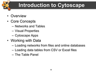
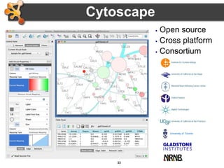
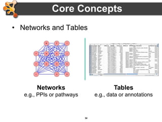
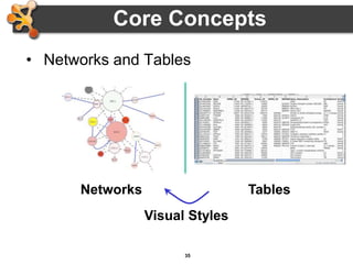
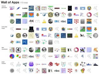
Alex Pico
Gladstone Institutes
San Francisco, CA
April 21, 2016
2
Outline
• Biological Networks
– Why Networks?
– Biological Network Taxonomy
– Analytical Approaches
– Visualization
• Break
• Introduction to Cytoscape
• Hands on Tutorial
– Data import
– Layout and apps
3
Why Networks?
• Networks are…
• Commonly understood
• Structured to reduce complexity
• More efficient than tables
• Network tools allow…
Analysis
• Characterize network properties
• Identify hubs and subnets
• Classify, quantify and correlate, e.g.,
cluster nodes by associated data
Visualization
• Explore data overlays
• Interpret mechanisms, e.g., how a process
is modulated or attenuated by a stimulus
4
Applications of Network Biology
jActiveModules, UCSD
PathBlast, UCSD
mCode, University of Toronto
DomainGraph, Max Planck Institute
• Gene Function Prediction
shows connections to sets of
genes/proteins involved in same
biological process
• Detection of protein
complexes/subnetworks
discover modularity & higher
order organization (motifs,
feedback loops)
• Network evolution
biological process(s)
conservation across species
• Prediction of interactions &
functional associations
statistically significant domain-
domain correlations in protein
interaction network to predict
protein-protein or genetic
interaction
5
Applications in Disease
• Identification of disease
subnetworks – identification
of disease network subnetworks
that are transcriptionally active
in disease.
• Subnetwork-based
diagnosis – source of
biomarkers for disease
classification, identify
interconnected genes whose
aggregate expression levels are
predictive of disease state
• Subnetwork-based gene
association – map common
pathway mechanisms affected
by collection of genotypes
(SNP, CNV)
Agilent Literature Search
Mondrian, MSKCC
PinnacleZ, UCSD
6
The Challenge
http://cytoscape-publications.tumblr.com/archive
7
Biological Network Taxonomy
• Pathways
– Signaling, Metabolic, Regulatory, etc
8
Biological Network Taxonomy
• Interactions
– Protein-Protein
– Protein-Ligand
– Domain-Domain
– Others
• Residue or atomic
• Cell-cell
• Epidemiology
• Social networks
9
Biological Network Taxonomy
• Similarity
– Protein-Protein
– Chemical similarity
– Ligand similarity (SEA)
– Others
• Tag clouds
• Topic maps
10
Biological Network Taxonomy
Where do I get the network?
There is no such thing!
550 different interaction databases!
… in 2013
It depends on your biological question
and your analysis plan.
11
The levels of organization of
complex networks:
 Node degree provides
information about single nodes
 Three or more nodes represent
a motif
 Larger groups of nodes are
called modules or
communities
 Hierarchy describes how the
various structural elements are
combined
Analytical Approaches
12
Analytical Approaches
Piñero, Sci Rep, 15 April 2016
13
Network topology statistics
such as node degree, degree
distribution, centralitiy,
clustering coefficient, shortest
paths, and robustness of the
network to the random removal
of single nodes are important
network characteristics.
Motif analysis is the
identification of small network
patterns that are over-
represented when compared
with a randomized version of
the same network. Regulatory
elements are often composed
of such motifs.
Analytical Approaches
Modularity refers to the
identification of sub-networks of
interconnected nodes that might
represent molecules physically
or functionally linked that work
coordinately to achieve a
specific function.
Network alignment and
comparison tools can identify
similarities between networks
and have been used to study
evolutionary relationships
between protein networks of
organisms.
14
• Concepts
– Graph/Network correspondence
– Node/Vertex correspondence
– Edge directedness
• Usually a network property
– Node degree
– Multigraph
• Allow multiple edges between nodes
– Hypergraph
• Allow edges to connect more than 2 nodes
Analytical Approaches
15
• Network measures
– Node degree
• Indegree: # of edges for which this node is a target
• Outdegree: # of edges for which this node is a
source
– Hub
• node with an exceptionally high degree
– Shortest path length
• Shortest traversal distance between two nodes
• Can be weighted if edges have weights or hops if not
Analytical Approaches
16
• Scale-free networks
– Degree distribution follows power law:
P(k) ~ k-γ, where γ is a constant.
– Result is that there are distinctive “hubs”
(essential proteins?)
– Overall, though, network is resilient to
perturbation
– Biological (and social) networks tend to be
scale-free
Analytical Approaches
17
Analytical Approaches
• Small-world networks
– any two arbitrary nodes are connected
by a small number of intermediate
edges
– the network has an average shortest
path length much smaller than the
number of nodes in the network
(Watts, Nature, 1998).
– Interaction networks have been shown
to be small-world networks (Barabási,
Nature Reviews in Genetics, 2004)
18
• Random networks
– homogeneous, nodes have similar degrees,
and not robust to arbitrary node failure
– Algorithms exist to create random networks
• Flat random network: Erdos-Renyi
• Scale-free: Barabasi-Albert
• Small-world (high clustering): Watts-Strogatz
– Useful to compare your network vs. a random
network
Analytical Approaches
19
• Network measures
– Clustering coefficient
• Measures how close the neighbors of a node are to
being a clique (fully connected group)
• # of edges connecting a node’s neighbors/the node’s
degree
0.5
1.0
0
0.3
Analytical Approaches
20
• Centrality - measures of node importance
– Degree centrality (find hubs)
• Degree of this node / (# of nodes – 1)
– Betweenness centrality (bottleneck)
• The average number of shortest paths that go
through this node / (# of pairs)
– Closeness centrality
• The sum of all shortest paths between this node
and all other nodes / (# of nodes – 1)
Analytical Approaches
21
• Motif finding
– Search directed networks for network motifs
(feed-forward loops, feedback loops, etc.)
Analytical Approaches
22
• Overrepresentation analysis
– Find terms (GO) that are statistically
overrepresented in a network
– Not really a network analysis technique
– Very useful for visualization
Analytical Approaches
23
• Clustering (find hubs, complexes)
– Goal: group related items together
• Clustering types:
– Hierarchical clustering
• Divide network into pair-wise hierarchy
– K-Means clustering
• Divide network into k groups
– MCL
• Uses a flow simulation to find groups
– Community Clustering
• Maximize intra-cluster edges vs. inter-cluster edges
Analytical Approaches
24
Visualization of Biological Networks
• Data Mapping
• Layouts
• Animation
25
Depiction
• Various ways to depict biological networks:
– Node-Link (graph) representation
– Partitioned Node-Link representation
– Matrix representation
• Can be useful for very dense networks
• Can also map information into cells of matrix
– e.g. degree, color scale (heat map)
– Hierarchical reduction to 1D
– Orthogonal 1D representation of nodes/edges
26
Data Mapping
• Mapping of data values associated with
graph elements onto graph visuals
• Visual attributes
– Node fill color, border color, border width, size,
shape, opacity, label
– Edge type, color, width, ending type, ending
size, ending color
• Mapping types
– Passthrough (labels)
– Continuous (numeric values)
– Discrete (categories)
27
• Avoid cluttering your visualization with too
much data
– Highlight meaningful differences
– Avoid confusing the viewer
– Consider creating multiple network images
Data Mapping
28
• Layouts determine the location of nodes and
(sometimes) the paths of edges
• Types:
– Simple
• Grid
• Partitions
– Hierarchical
• layout data as a tree or hierarchy
• Works best when there are no loops
– Circular (Radial)
• arrange nodes around a circle
• could use node attributes to govern position
– e.g. degree sorted
Layouts
29
• Types:
– Force-Directed
• simulate edges as springs
• may be weighted or unweighted
– Combining layouts
• Use a general layout (force directed) for the entire
graph, but use hierarchical or radial to focus on a
particular portion
– Multi-layer layouts
• Partition graph, layout each partition then layout
partitions
– Many, many others
Layouts
30
• Use layouts to convey the relationships
between the nodes.
• Layout algorithms may need to be “tuned”
to fit your network.
• There is not one correct layout. Try different
things.
Layouts
31
Animation
• Animation is useful to show changes in a
network:
– Over a time series
– Over different conditions
– Between species
32
Introduction to Cytoscape
• Overview
• Core Concepts
– Networks and Tables
– Visual Properties
– Cytoscape Apps
• Working with Data
– Loading networks from files and online databases
– Loading data tables from CSV or Excel files
– The Table Panel
33
 Open source
 Cross platform
 Consortium
Cytoscape
University of Toronto
34
Core Concepts
• Networks and Tables
Tables
e.g., data or annotations
Networks
e.g., PPIs or pathways
35
Core Concepts
• Networks and Tables
TablesNetworks
Visual Styles
36
Core Concepts
• Cytoscape Apps!
apps.cytoscape.org
37
Loading Networks
• Use import network from file
– Excel file
– Comma or tab delimited text
38
Loading Networks
• But what if I don’t have a network?!
39
Loading Tables
• Nodes and edges can have
data associated with them
– Gene expression data
– Mass spectrometry data
– Protein structure information
– Gene Ontology terms, etc.
• Cytoscape supports multiple
data types: Numbers, Text,
Boolean, Lists...
40
• Use import table from file
– Excel file
– Comma or tab delimited text
Loading Tables
41
Visual Style Manager
• Click on the Styles tab
42
• Click on Select tab
Selection Filters
43
• Sessions save everything as .cys files:
Networks, Tables, Styles, Screen sizes, etc
• Export networks in different formats:
SIF, GML, XGMML, BioPAX, PSI-MI 1 & 2.5
• Publication quality graphics in several formats:
PDF, EPS, SVG, PNG, JPEG, and BMP
Saving and Exporting
44
Getting Help
45
Tips & Tricks
• Network Collections
– Each collection has a “root” network
– Changing the attribute for a node in one
network will also change that attribute for a
node with the same SUID in all other networks
within the collection
– You can clone a network into a new collection
to “decouple” it and start a new root
46
• Network views
– When you open a large network, you will not
get a view by default
– To improve interactive performance, Cytoscape
has the concept of “Levels of Detail”
• Some visual attributes will only be apparent when
you zoom in
• The level of detail for various attributes can be
changed in the preferences
• To see what things will look like at full detail:
– ViewShow Graphics Details
Tips & Tricks
47
• Sessions
– Sessions save pretty much everything:
• Networks
• Properties
• Visual styles
• Screen sizes
– Saving a session on a large screen may require
some resizing when opened on your laptop
Tips & Tricks
48
• Task monitor
– Current task displayed in status bar (lower left)
– Icon opens complete task history
• Memory
– Current status (lower right)
– Toggle open for details and “Free Unused
Memory” button
Tips & Tricks
49
• CytoscapeConfiguration directory
– Your defaults and any apps downloaded from the
App Store will go here
• App Manager
– This is where you search/install/update/uninstall
apps
– You now have the option of disabling vs.
uninstalling…
– Can also install and update apps directly from the
App Store website, if you have Cytoscape 3 up and
running
Tips & Tricks
50
Cytoscape: Platform
• Cytoscape as a platform
– App architecture
• http://apps.cytoscape.org
– Use cases
• Expression data analysis
• Protein complexes
• Agilent literature search
51
Hands-on Tutorial
Introduction to Cytoscape:
Networks, Data, Styles, Layouts and App Manager
tutorials.cytoscape.org

2016 Cytoscape 3.3 Tutorial

  • 1.
    Alex Pico Gladstone Institutes SanFrancisco, CA April 21, 2016
  • 2.
    2 Outline • Biological Networks –Why Networks? – Biological Network Taxonomy – Analytical Approaches – Visualization • Break • Introduction to Cytoscape • Hands on Tutorial – Data import – Layout and apps
  • 3.
    3 Why Networks? • Networksare… • Commonly understood • Structured to reduce complexity • More efficient than tables • Network tools allow… Analysis • Characterize network properties • Identify hubs and subnets • Classify, quantify and correlate, e.g., cluster nodes by associated data Visualization • Explore data overlays • Interpret mechanisms, e.g., how a process is modulated or attenuated by a stimulus
  • 4.
    4 Applications of NetworkBiology jActiveModules, UCSD PathBlast, UCSD mCode, University of Toronto DomainGraph, Max Planck Institute • Gene Function Prediction shows connections to sets of genes/proteins involved in same biological process • Detection of protein complexes/subnetworks discover modularity & higher order organization (motifs, feedback loops) • Network evolution biological process(s) conservation across species • Prediction of interactions & functional associations statistically significant domain- domain correlations in protein interaction network to predict protein-protein or genetic interaction
  • 5.
    5 Applications in Disease •Identification of disease subnetworks – identification of disease network subnetworks that are transcriptionally active in disease. • Subnetwork-based diagnosis – source of biomarkers for disease classification, identify interconnected genes whose aggregate expression levels are predictive of disease state • Subnetwork-based gene association – map common pathway mechanisms affected by collection of genotypes (SNP, CNV) Agilent Literature Search Mondrian, MSKCC PinnacleZ, UCSD
  • 6.
  • 7.
    7 Biological Network Taxonomy •Pathways – Signaling, Metabolic, Regulatory, etc
  • 8.
    8 Biological Network Taxonomy •Interactions – Protein-Protein – Protein-Ligand – Domain-Domain – Others • Residue or atomic • Cell-cell • Epidemiology • Social networks
  • 9.
    9 Biological Network Taxonomy •Similarity – Protein-Protein – Chemical similarity – Ligand similarity (SEA) – Others • Tag clouds • Topic maps
  • 10.
    10 Biological Network Taxonomy Wheredo I get the network? There is no such thing! 550 different interaction databases! … in 2013 It depends on your biological question and your analysis plan.
  • 11.
    11 The levels oforganization of complex networks:  Node degree provides information about single nodes  Three or more nodes represent a motif  Larger groups of nodes are called modules or communities  Hierarchy describes how the various structural elements are combined Analytical Approaches
  • 12.
  • 13.
    13 Network topology statistics suchas node degree, degree distribution, centralitiy, clustering coefficient, shortest paths, and robustness of the network to the random removal of single nodes are important network characteristics. Motif analysis is the identification of small network patterns that are over- represented when compared with a randomized version of the same network. Regulatory elements are often composed of such motifs. Analytical Approaches Modularity refers to the identification of sub-networks of interconnected nodes that might represent molecules physically or functionally linked that work coordinately to achieve a specific function. Network alignment and comparison tools can identify similarities between networks and have been used to study evolutionary relationships between protein networks of organisms.
  • 14.
    14 • Concepts – Graph/Networkcorrespondence – Node/Vertex correspondence – Edge directedness • Usually a network property – Node degree – Multigraph • Allow multiple edges between nodes – Hypergraph • Allow edges to connect more than 2 nodes Analytical Approaches
  • 15.
    15 • Network measures –Node degree • Indegree: # of edges for which this node is a target • Outdegree: # of edges for which this node is a source – Hub • node with an exceptionally high degree – Shortest path length • Shortest traversal distance between two nodes • Can be weighted if edges have weights or hops if not Analytical Approaches
  • 16.
    16 • Scale-free networks –Degree distribution follows power law: P(k) ~ k-γ, where γ is a constant. – Result is that there are distinctive “hubs” (essential proteins?) – Overall, though, network is resilient to perturbation – Biological (and social) networks tend to be scale-free Analytical Approaches
  • 17.
    17 Analytical Approaches • Small-worldnetworks – any two arbitrary nodes are connected by a small number of intermediate edges – the network has an average shortest path length much smaller than the number of nodes in the network (Watts, Nature, 1998). – Interaction networks have been shown to be small-world networks (Barabási, Nature Reviews in Genetics, 2004)
  • 18.
    18 • Random networks –homogeneous, nodes have similar degrees, and not robust to arbitrary node failure – Algorithms exist to create random networks • Flat random network: Erdos-Renyi • Scale-free: Barabasi-Albert • Small-world (high clustering): Watts-Strogatz – Useful to compare your network vs. a random network Analytical Approaches
  • 19.
    19 • Network measures –Clustering coefficient • Measures how close the neighbors of a node are to being a clique (fully connected group) • # of edges connecting a node’s neighbors/the node’s degree 0.5 1.0 0 0.3 Analytical Approaches
  • 20.
    20 • Centrality -measures of node importance – Degree centrality (find hubs) • Degree of this node / (# of nodes – 1) – Betweenness centrality (bottleneck) • The average number of shortest paths that go through this node / (# of pairs) – Closeness centrality • The sum of all shortest paths between this node and all other nodes / (# of nodes – 1) Analytical Approaches
  • 21.
    21 • Motif finding –Search directed networks for network motifs (feed-forward loops, feedback loops, etc.) Analytical Approaches
  • 22.
    22 • Overrepresentation analysis –Find terms (GO) that are statistically overrepresented in a network – Not really a network analysis technique – Very useful for visualization Analytical Approaches
  • 23.
    23 • Clustering (findhubs, complexes) – Goal: group related items together • Clustering types: – Hierarchical clustering • Divide network into pair-wise hierarchy – K-Means clustering • Divide network into k groups – MCL • Uses a flow simulation to find groups – Community Clustering • Maximize intra-cluster edges vs. inter-cluster edges Analytical Approaches
  • 24.
    24 Visualization of BiologicalNetworks • Data Mapping • Layouts • Animation
  • 25.
    25 Depiction • Various waysto depict biological networks: – Node-Link (graph) representation – Partitioned Node-Link representation – Matrix representation • Can be useful for very dense networks • Can also map information into cells of matrix – e.g. degree, color scale (heat map) – Hierarchical reduction to 1D – Orthogonal 1D representation of nodes/edges
  • 26.
    26 Data Mapping • Mappingof data values associated with graph elements onto graph visuals • Visual attributes – Node fill color, border color, border width, size, shape, opacity, label – Edge type, color, width, ending type, ending size, ending color • Mapping types – Passthrough (labels) – Continuous (numeric values) – Discrete (categories)
  • 27.
    27 • Avoid clutteringyour visualization with too much data – Highlight meaningful differences – Avoid confusing the viewer – Consider creating multiple network images Data Mapping
  • 28.
    28 • Layouts determinethe location of nodes and (sometimes) the paths of edges • Types: – Simple • Grid • Partitions – Hierarchical • layout data as a tree or hierarchy • Works best when there are no loops – Circular (Radial) • arrange nodes around a circle • could use node attributes to govern position – e.g. degree sorted Layouts
  • 29.
    29 • Types: – Force-Directed •simulate edges as springs • may be weighted or unweighted – Combining layouts • Use a general layout (force directed) for the entire graph, but use hierarchical or radial to focus on a particular portion – Multi-layer layouts • Partition graph, layout each partition then layout partitions – Many, many others Layouts
  • 30.
    30 • Use layoutsto convey the relationships between the nodes. • Layout algorithms may need to be “tuned” to fit your network. • There is not one correct layout. Try different things. Layouts
  • 31.
    31 Animation • Animation isuseful to show changes in a network: – Over a time series – Over different conditions – Between species
  • 32.
    32 Introduction to Cytoscape •Overview • Core Concepts – Networks and Tables – Visual Properties – Cytoscape Apps • Working with Data – Loading networks from files and online databases – Loading data tables from CSV or Excel files – The Table Panel
  • 33.
    33  Open source Cross platform  Consortium Cytoscape University of Toronto
  • 34.
    34 Core Concepts • Networksand Tables Tables e.g., data or annotations Networks e.g., PPIs or pathways
  • 35.
    35 Core Concepts • Networksand Tables TablesNetworks Visual Styles
  • 36.
    36 Core Concepts • CytoscapeApps! apps.cytoscape.org
  • 37.
    37 Loading Networks • Useimport network from file – Excel file – Comma or tab delimited text
  • 38.
    38 Loading Networks • Butwhat if I don’t have a network?!
  • 39.
    39 Loading Tables • Nodesand edges can have data associated with them – Gene expression data – Mass spectrometry data – Protein structure information – Gene Ontology terms, etc. • Cytoscape supports multiple data types: Numbers, Text, Boolean, Lists...
  • 40.
    40 • Use importtable from file – Excel file – Comma or tab delimited text Loading Tables
  • 41.
    41 Visual Style Manager •Click on the Styles tab
  • 42.
    42 • Click onSelect tab Selection Filters
  • 43.
    43 • Sessions saveeverything as .cys files: Networks, Tables, Styles, Screen sizes, etc • Export networks in different formats: SIF, GML, XGMML, BioPAX, PSI-MI 1 & 2.5 • Publication quality graphics in several formats: PDF, EPS, SVG, PNG, JPEG, and BMP Saving and Exporting
  • 44.
  • 45.
    45 Tips & Tricks •Network Collections – Each collection has a “root” network – Changing the attribute for a node in one network will also change that attribute for a node with the same SUID in all other networks within the collection – You can clone a network into a new collection to “decouple” it and start a new root
  • 46.
    46 • Network views –When you open a large network, you will not get a view by default – To improve interactive performance, Cytoscape has the concept of “Levels of Detail” • Some visual attributes will only be apparent when you zoom in • The level of detail for various attributes can be changed in the preferences • To see what things will look like at full detail: – ViewShow Graphics Details Tips & Tricks
  • 47.
    47 • Sessions – Sessionssave pretty much everything: • Networks • Properties • Visual styles • Screen sizes – Saving a session on a large screen may require some resizing when opened on your laptop Tips & Tricks
  • 48.
    48 • Task monitor –Current task displayed in status bar (lower left) – Icon opens complete task history • Memory – Current status (lower right) – Toggle open for details and “Free Unused Memory” button Tips & Tricks
  • 49.
    49 • CytoscapeConfiguration directory –Your defaults and any apps downloaded from the App Store will go here • App Manager – This is where you search/install/update/uninstall apps – You now have the option of disabling vs. uninstalling… – Can also install and update apps directly from the App Store website, if you have Cytoscape 3 up and running Tips & Tricks
  • 50.
    50 Cytoscape: Platform • Cytoscapeas a platform – App architecture • http://apps.cytoscape.org – Use cases • Expression data analysis • Protein complexes • Agilent literature search
  • 51.
    51 Hands-on Tutorial Introduction toCytoscape: Networks, Data, Styles, Layouts and App Manager tutorials.cytoscape.org

Editor's Notes

  • #3 EDIT: schedule
  • #5 Gene Function Prediction – basic but important, examining genes (proteins) in a network context shows connections to sets of genes/proteins involved in same biological process that are likely to function in that process Detection of protein complexes/other modular structures – although interaction networks are based on pair-wise interactions, there is clear evidence for modularity & higher order organization (motifs, feedback loops) Network evolution – biological process(s) conservation across species (PathBLAST, NetworkBLAST to align p-p interaction networks & clusters) Prediction of new interactions and functional associations – Statistically significant domain-domain correlations in protein interaction network suggest that certain domain (and domain pairs) mediate protein binding. Machine learning extends this to suggest to predict protein-protein or genetic interaction through integration of diverse types of evidence for interaction
  • #6 Identification of disease subnetworks – identification of disease network subnetworks that are transcriptionally active in disease. These suggest key pathway components in disease progression and provide leads for further study and potential therapeutic targets Subnetwork-based diagnosis – subnetworks also provide a rich source of biomarkers for disease classification, based on mRNA profiling integrated with protein networks to identify subnetwork biomarkers (interconnected genes whose aggregate expression levels are predictive of disease state) Subnetwork-based gene association – molecular networks will provide a powerful framework for mapping common pathway mechanisms affected by collection of genotypes (SNP, CNV)
  • #7 Some good examples An example with perhaps too many visual properties Cool cell illustration Mapping brain regions (not proteins!) Cytoscape is often just one part of an analysis pipeline
  • #8 Signaling pathway: Interleukin-2 Metabolic pathway: Krebs (TCA) Cycle
  • #13 “Cancer genes are central not only in terms of number of neighbors, but also in terms of the clusters they connect. Remarkably, we found that high Participation roles played by cancer genes are not explained by their higher number of interactions, but by their unique inter-modular connectivity patterns. We also found that these connectivity patterns differ for disease genes with contrasting inheritance modes: while autosomal dominant genes play high participation roles, autosomal recessive genes are more confined to their own modules. “ Replicates over 6 different interaction networks (HIPPIE18, BIANA40, BioGRID41, IntAct42, IrefIndex43 and from Human Interactome Project (HBI)19,44). Looked at ~2000 Mendelian disease genes and 781 “cancer driver genes.”
  • #23 Note: all Cytoscape ORA tools provide a network visualization of terms and a ranked table with statistics
  • #26 Last two: - NetGestalt (used to align data in fashion of genome browsers) - BioFrabric (used to organize/explore massive hairballs)
  • #32 http://git.dhimmel.com/SIDER2/similarity/
  • #33 EDIT: according to schedule
  • #34 NOTE: Pre-acknowledgements slide
  • #35 Notes: it is a Cytoscape goal that both the graph model and the data are free from Biological semantics
  • #37 Screenshots: App Store front page, example app, and wall of apps Note: mention increasing number of apps (and ports to 3.x) Alternative: visit App Store live 272 apps – April 2016
  • #39 Welcome! - web services: a couple provided by default (more in App Store) - preset networks from BioGRID per species (mouse over for details)
  • #42 New interface! - def, map, byp - example continuous mapping panel - menu of provided visual styles
  • #49 Note: these used to be major issues in 2.x