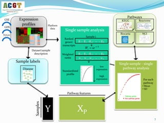
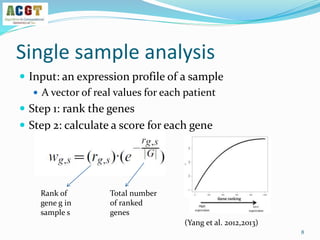
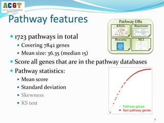
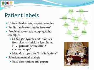
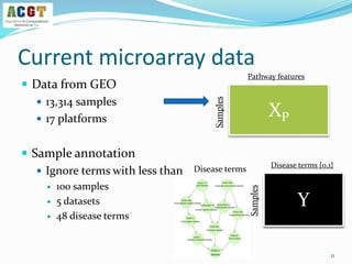
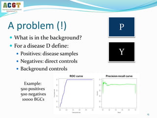
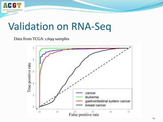
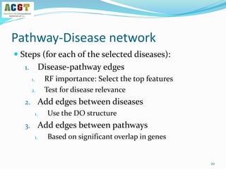
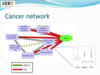
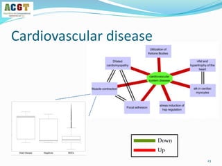
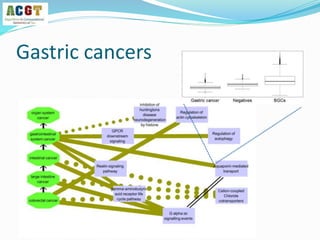
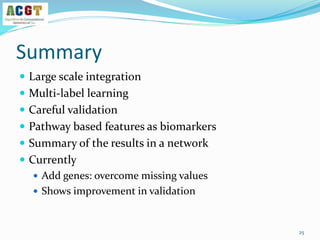
This document summarizes a study that integrated pathway and gene expression data from over 13,000 samples across 17 platforms to perform multi-label classification of 48 diseases. Pathway activity scores were calculated for each sample and used as features for classification, along with sample labels determined through manual dataset analysis. Classification was performed using multiple algorithms and validated through cross-validation and comparison to previous studies. Performance was improved over previous work, as shown by increased recall and precision. Relationships between diseases and pathways were also modeled in a network graph.

1. 1
David Amar, Tom Hait, and Ron Shamir
Blavatnik School of Computer Science
Tel Aviv University

2. 2

3. Comparative genomics
 Standard expression experiments: cases vs. controls ->
differential genes -> interpretation
 Problems
 Small number of samples
 Non-specific signal
 Interpretation of a gene set/ gene ranking
 Goal: find specific changes for a tested disease
 E.g., an up-regulated pathway
 Crucial for clinical studies
3

4. Previous integrative classification studies
 Huang et al. 2010 PNAS (9,160 samples); Schmid et al.
PNAS 2012 (3,030); Lee et al. Bioinformatics 2013 (~14,000)
 Multilabel classification
 Global expression patterns
 Only 1-3 platforms
 Many datasets were removed from GEO
 No “healthy” class (Huang);No diseases (Lee)
 Pathprint (Altschuler et al. 2013)
 Use pathways
 Tissue classification (as in Lee et al.)
4

5. Integrating pathways and molecular
profiles
 Enrichment tests
 Improves interpretability
 GSEAGSA
 Ranked based
 Higher statistical power
 Classification
 Extract pathway features
 Example: given a pathway remove non-differential genes
 Not clear if prediction performance improves
compared to using genes (Staiger et al. 2013)
5

6. 6

7. Pathways
KEGG Reactome
Biocarta NCI
Expression
profiles
GSE
GDS
TCGA
Sample labels
Disease
Datasetsample
description
Single sample - single
pathway analysis
For each
pathway
• Mean
• SD
Y
Samples
XP
Pathway features
Platform
data
Single sample analysis
Ranked
genes
transcripts
Sample j
Weighted
ranks
/i k
iW ie

Standardized
profile
low
expression
high
expression
7

8. Single sample analysis
 Input: an expression profile of a sample
 A vector of real values for each patient
 Step 1: rank the genes
 Step 2: calculate a score for each gene
Rank of
gene g in
sample s
Total number
of ranked
genes
(Yang et al. 2012,2013)
8

9. Pathway features
 1723 pathways in total
 Covering 7842 genes
 Mean size: 36.35 (median 15)
 Score all genes that are in the pathway databases
 Pathway statistics:
 Mean score
 Standard deviation
 Skewness
 KS test
Pathway DBs
KEGG Reactome
Biocarta NCI
9

10. Patient labels
 Unite ~180 datasets, >14,000 samples
 Public databases contain ‘free text’
 Problem: automatic mapping fails,
example:
 GDS4358:” lymph-node biopsies
from classic Hodgkins lymphoma
HIV- patients before ABVD
chemotherapy”
 MetaMap top score: “HIV infections”
 Solution: manual analysis
 Read descriptions and papers
10

11. Current microarray data
 Data from GEO
 13,314 samples
 17 platforms
 Sample annotation
 Ignore terms with less than
 100 samples
 5 datasets
 48 disease terms
Disease terms
XP
Samples
Pathway features
Y
Disease terms {0,1}
Samples 11

12. 12

13. Multi-label classification algorithms
 Learn a single classifier for each disease
 Ignore class dependencies
 Adaptation: Bayesian Correction
 Learn single classifiers
 Correct errors using the DO DAG
 Transformation: use the label power
sets and learn a multiclass model
 Using RF: multi-label trees
 Was better than most approaches in an
experimental study (Madjarov et al. 2012)
13

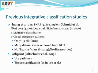
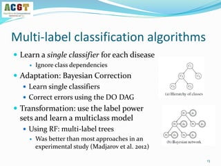
14. How to validate an classifier?
 Use leave-dataset out cross-validation
 Global AUC scores: each prediction Pij vs the correct label Yij
 Disease based AUC scores: consider each column separately
14
Y
Disease terms {0,1}
Samples
P
Probabilities [0,1]
Samples
The output of a multi-label learner
Test set

15. A problem (!)
 What is in the background?
 For a disease D define:
 Positives: disease samples
 Negatives: direct controls
 Background controls
15
Example:
500 positives
500 negatives
10000 BGCs
Y
P

16. Multistep validation
16
 It is recommended to use several scores (Lee et al. 2013)
 Measure global AUPR
 For each disease we calculate three scores
Measure Used (additional)
information
AUPR: check separation between positives and
all others
Sick vs. not sick
ROC: test for separation between positives and
negatives
Direct use of negatives
Meta analysis p-value: calculate the overall
separation significance within the original
datasets (a p-value)
Mapping of samples to
datasets

17. Performance results
17
Meta analysis q-value < 0.001 (filled boxes)
Positives vs. negatives ROC
AUPR

18. Performance results
18
8.5% improvement in
recall, 12% in precision,
compared to Huang et al.

19. Validation on RNA-Seq
Data from TCGA: 1,699 samples
19

20. Pathway-Disease network
 Steps (for each of the selected diseases):
1. Disease-pathway edges
1. RF importance: Select the top features
2. Test for disease relevance
2. Add edges between diseases
1. Use the DO structure
3. Add edges between pathways
1. Based on significant overlap in genes
20

21. Cancer network
Down
Up

22. Cardiovascular disease
23
Down
Up

23. Gastric cancers

24. Summary
 Large scale integration
 Multi-label learning
 Careful validation
 Pathway based features as biomarkers
 Summary of the results in a network
 Currently
 Add genes: overcome missing values
 Shows improvement in validation
25

25. Acknowledgements
 Ron Shamir
 Tom Hait