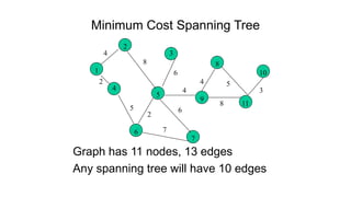
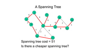
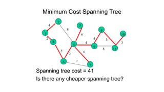
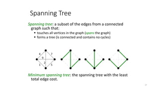
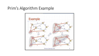
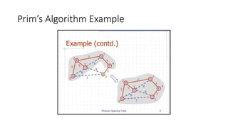
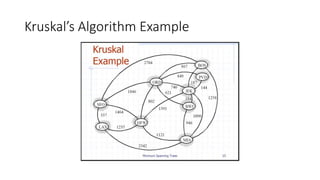
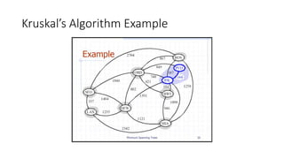
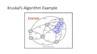
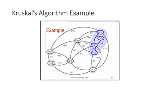
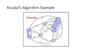
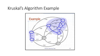
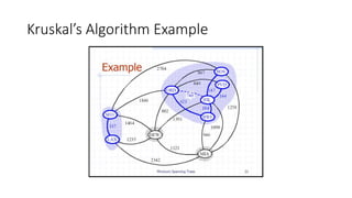
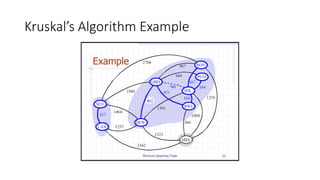
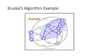
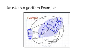
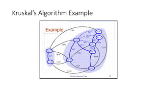
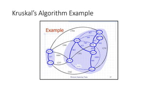
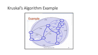
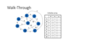
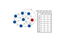
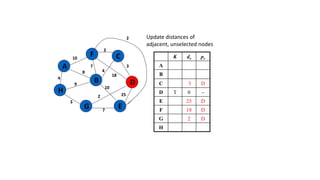
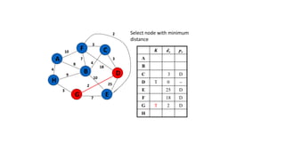
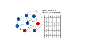
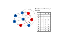
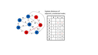
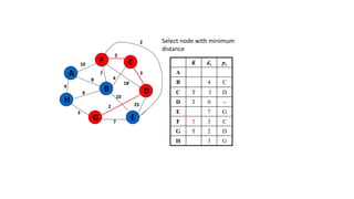
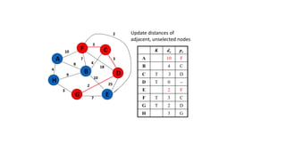
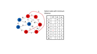
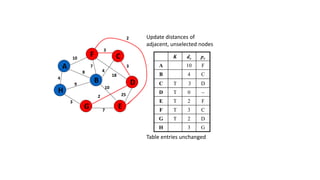
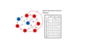
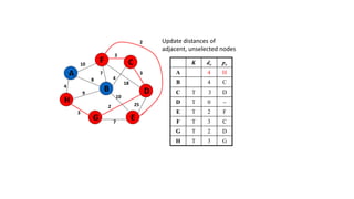
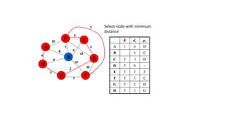
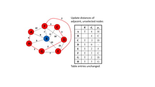
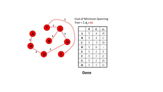
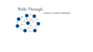
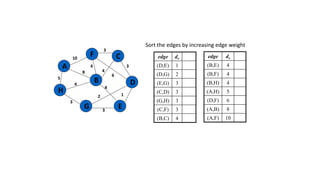
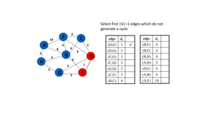
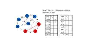
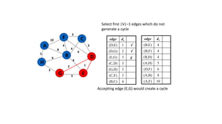
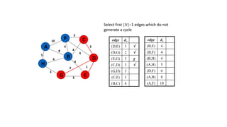
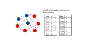
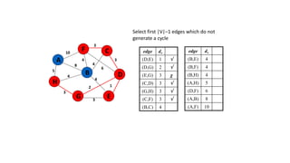
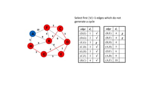
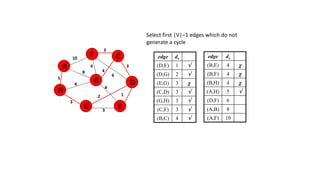
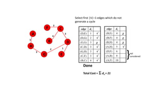
The document discusses minimum spanning trees (MSTs) and algorithms for finding them. It defines an MST as a subgraph of an undirected weighted graph that spans all nodes, is connected, acyclic, and has the minimum total edge weight among all spanning trees. The document explains Prim's and Kruskal's algorithms for finding MSTs and provides examples of how they work on sample graphs. It also discusses properties of MSTs such as that multiple MSTs may exist for a given graph.

2. 2
Paths and cycles
• A path is a sequence of nodes
v1, v2, …, vN such that (vi,vi+1)E for 0<i<N
• The length of the path is N-1.
• Simple path: all vi are distinct, 0<i<N
• A cycle is a path such that v1=vN
• An acyclic graph has no cycles

3. 3
Cycles
PIT
BOS
JFK
DTW
LAX
SFO

4. 4
More useful definitions
• In a directed graph:
• The indegree of a node v is the number of distinct edges (w,v)E.
• The outdegree of a node v is the number of distinct edges (v,w)E.
• A node with indegree 0 is a root.

5. 5
Trees are graphs
• A dag is a directed acyclic graph.
• A tree is a connected acyclic undirected graph.
• A forest is an acyclic undirected graph (not necessarily connected),
i.e., each connected component is a tree.

6. Tree
• Connected graph that has no cycles
• n vertex connected graph with n-1
edges

7. Spanning Tree
• Subgraph that includes all vertices of
the original graph
• Subgraph is a tree
• If original graph has n vertices, the
spanning tree has n vertices and n-1
edges

8. Minimum Cost Spanning Tree
• Weighted, undirected graph G
• Spanning tree T of G
• Cost(T) = sum of edge weights
• MST = Spanning tree T of G such
that no other spanning tree T' of G
has cost(T') < cost(T)

9. Minimum Cost Spanning Tree
Graph has 11 nodes, 13 edges
Any spanning tree will have 10 edges
2
3
8
101
4
5
9
11
6
7
4
8
6
6
7
5
2
4
4 5
3
8
2

10. A Spanning Tree
Spanning tree cost = 51
Is there a cheaper spanning tree?
2
3
8
101
4
5
9
11
6
7
4
8
6
6
7
5
2
4
4 5
3
8
2

11. Minimum Cost Spanning Tree
Spanning tree cost = 41
Is there any cheaper spanning tree?
2
3
8
101
4
5
9
11
6
7
4
8
6
6
7
5
2
4
4 5
3
8
2

12. 12
Edsger Wybe Dijkstra
(1930-2002)
• Invented concepts of structured programming,
synchronization, weakest precondition, and "semaphores"
for controlling computer processes. The Oxford English
Dictionary cites his use of the words "vector" and "stack" in
a computing context.
• Believed programming should be taught without computers
• 1972 Turing Award
• “In their capacity as a tool, computers will be but a ripple on
the surface of our culture. In their capacity as intellectual
challenge, they are without precedent in the cultural history
of mankind.”

13. 13
Dijkstra’s Algorithm for
Single Source Shortest Path
• Classic algorithm for solving shortest path in weighted graphs (with
only positive edge weights)
• Similar to breadth-first search, but uses a priority queue instead of a
FIFO queue:
• Always select (expand) the vertex that has a lowest-cost path to the start
vertex
• a kind of “greedy” algorithm
• Correctly handles the case where the lowest-cost (shortest) path to a
vertex is not the one with fewest edges

14. 14
void BFS(Node startNode) {
Queue s = new Queue;
for v in Nodes do
v.visited = false;
startNode.dist = 0;
s.enqueue(startNode);
while (!s.empty()) {
x = s.dequeue();
for y in x.children() do
if (x.dist+1<y.dist) {
y.dist = x.dist+1;
s.enqueue(y);
}
}
}
void shortestPath(Node startNode) {
Heap s = new Heap;
for v in Nodes do
v.dist = ;
s.insert(v);
startNode.dist = 0;
s.decreaseKey(startNode);
startNode.previous = null;
while (!s.empty()) {
x = s.deleteMin();
for y in x.children() do
if (x.dist+c(x,y) < y.dist) {
y.dist = x.dist+c(x,y);
s.decreaseKey(y);
y.previous = x;
}
}
}

15. 15
Dijkstra’s Algorithm:
Correctness Proof
Let Known be the set of nodes that were extracted from the heap
(through deleteMin)
• For every node x, x.dist = the cost of the shortest path from startNode
to x going only through nodes in Known
• In particular, if x in Known then x.dist = the shortest path cost
• Once a node x is in Known, it will never be reinserted into the heap

16. 16
Dijkstra’s Algorithm:
Correctness Proof
startNode
Known
x.dist

17. 17
Dijkstra’s Algorithm in Action
A
C
B
D
F H
G
E
2 2 3
2
1
1
4
10
8
1
1
9
4
2
7

18. 18
Dijkstra’s Algorithm in Action
A
C
B
D
F H
G
E
2 2 3
2
1
1
4
10
8
1
1
9
4
2
7
0
8



9

next

19. 19
Dijkstra’s Algorithm in Action
A
C
B
D
F H
G
E
2 2 3
2
1
1
4
10
8
1
1
9
4
2
7
0
8
9


9
15
next

20. 20
Dijkstra’s Algorithm in Action
A
C
B
D
F H
G
E
2 2 3
2
1
1
4
10
8
1
1
9
4
2
7
0
8
9


119
13
next

21. 21
Dijkstra’s Algorithm in Action
A
C
B
D
F H
G
E
2 2 3
2
1
1
4
10
8
1
1
9
4
2
7
0
8
9

11
119
13
next

22. 22
Dijkstra’s Algorithm in Action
A
C
B
D
F H
G
E
2 2 3
2
1
1
4
10
8
1
1
9
4
2
7
0
8
9

11
119
13
next

23. 23
Dijkstra’s Algorithm in Action
A
C
B
D
F H
G
E
2 2 3
2
1
1
4
10
8
1
1
9
4
2
7
0
8
9
14
11
119
13
next

24. 24
Dijkstra’s Algorithm in Action
A
C
B
D
F H
G
E
2 2 3
2
1
1
4
10
8
1
1
9
4
2
7
0
8
9
14
11
119
13
next

25. 25
Dijkstra’s Algorithm in Action
A
C
B
D
F H
G
E
2 2 3
2
1
1
4
10
8
1
1
9
4
2
7
0
8
9
14
11
119
13
Done

26. 26
Data Structures
for Dijkstra’s Algorithm
Select the unknown node with the lowest cost
findMin/deleteMin
y’s cost = min(y’s old cost, …)
decreaseKey
|V| times:
|E| times:
runtime: O((|V|+|E|) log |V|)
O(log |V|)
O(log |V|)

27. 27
Spanning tree: a subset of the edges from a connected
graph such that:
 touches all vertices in the graph (spans the graph)
 forms a tree (is connected and contains no cycles)
Minimum spanning tree: the spanning tree with the least
total edge cost.
Spanning Tree
4 7
1 5
9
2

28. 28
Applications of Minimal Spanning Trees
• Communication networks
• VLSI design
• Transportation systems

29. Minimum Spanning Trees
Text
Read Weiss, §9.5
Prim’s Algorithm
Weiss §9.5.1
Similar to Dijkstra’s Algorithm
Kruskal’s Algorithm
Weiss §9.5.2
Focuses on edges, rather than nodes

30. Definition
• A Minimum Spanning Tree (MST) is a subgraph of an undirected graph
such that the subgraph spans (includes) all nodes, is connected, is
acyclic, and has minimum total edge weight

32. Real Life Application of a MST
A cable TV company is laying cable in a new neighborhood. If it is
constrained to bury the cable only along certain paths, then there
would be a graph representing which points are connected by those
paths. Some of those paths might be more expensive, because they
are longer, or require the cable to be buried deeper; these paths
would be represented by edges with larger weights. A minimum
spanning tree would be the network with the lowest total cost.

33. 33
Problem: Laying Telephone Wire
Central office

34. 34
Wiring: Naïve Approach
Central office
Expensive!

35. 35
Wiring: Better Approach
Central office
Minimize the total length of wire connecting the customers

36. 36
Minimum Spanning Tree (MST)(see Weiss, Section 24.2.2)
• it is a tree (i.e., it is acyclic)
• it covers all the vertices V
– contains |V| - 1 edges
• the total cost associated with tree edges is the
minimum among all possible spanning trees
• not necessarily unique
A minimum spanning tree is a subgraph of an
undirected weighted graph G, such that

37. Algorithm Characteristics
• Both Prim’s and Kruskal’s Algorithms work with
undirected graphs
• Both work with weighted and unweighted graphs but
are more interesting when edges are weighted
• Both are greedy algorithms that produce optimal
solutions

38. MST
• A minimum spanning tree connects all nodes in a given graph
• A MST must be a connected and undirected graph
• A MST can have weighted edges
• Multiple MSTs can exist within a given undirected graph

39. More about Multiple MSTs
• Multiple MSTs can be generated depending on which algorithm is
used
• If you wish to have an MST start at a specific node
• However, if there are weighted edges and all weighted edges are
unique, only one MST will exist

40. Borůvka’s Algorithm
• The first MST Algorithm was created by Otakar Borůvka in 1926
• The algorithm was used to create efficient connections between the
electricity network in the Czech Republic
• No longer used since Prim’s and Kruskal’s algorithms were discovered

41. Prim’s Algorithm
• Initially discovered in 1930 by Vojtěch Jarník, then rediscovered in
1957 by Robert C. Prim
• Similar to Dijkstra’s Algorithm regarding a connected graph
• Starts off by picking any node within the graph and growing from
there

42. Prim’s Algorithm Cont.
• Label the starting node, A, with a 0 and all others with infinite
• Starting from A, update all the connected nodes’ labels to A with their
weighted edges if it less than the labeled value
• Find the next smallest label and update the corresponding connecting
nodes
• Repeat until all the nodes have been visited

43. Prim’s Algorithm Example

44. Prim’s Algorithm Example

45. Kruskal’s Algorithm
• Created in 1957 by Joseph Kruskal
• Finds the MST by taking the smallest weight in the graph and connecting the two
nodes and repeating until all nodes are connected to just one tree
• This is done by creating a priority queue using the weights as keys
• Each node starts off as it’s own tree
• While the queue is not empty, if the edge retrieved connects two trees, connect
them, if not, discard it
• Once the queue is empty, you are left with the minimum spanning tree

46. Kruskal’s Algorithm Example

47. Kruskal’s Algorithm Example

48. Kruskal’s Algorithm Example

49. Kruskal’s Algorithm Example

50. Kruskal’s Algorithm Example

51. Kruskal’s Algorithm Example

52. Kruskal’s Algorithm Example

53. Kruskal’s Algorithm Example

54. Kruskal’s Algorithm Example

55. Kruskal’s Algorithm Example

56. Kruskal’s Algorithm Example

57. Kruskal’s Algorithm Example

58. Kruskal’s Algorithm Example

59. Kruskal’s Algorithm Example

60. Prim’s Algorithm
• Similar to Dijkstra’s Algorithm except that dv records edge weights,
not path lengths

61. Walk-Through
Initialize array
K dv pv
A F  
B F  
C F  
D F  
E F  
F F  
G F  
H F  
4
25
A
H
B
F
E
D
C
G 7
2
10
18
3
4
3
7
8
9
3
10
2

62. 4
25
A
H
B
F
E
D
C
G 7
2
10
18
3
4
3
7
8
9
3
10
Start with any node, say D
K dv pv
A
B
C
D T 0 
E
F
G
H
2

63. 4
25
A
H
B
F
E
D
C
G 7
2
10
18
3
4
3
7
8
9
3
10
Update distances of
adjacent, unselected nodes
K dv pv
A
B
C 3 D
D T 0 
E 25 D
F 18 D
G 2 D
H
2

64. 4
25
A
H
B
F
E
D
C
G 7
2
10
18
3
4
3
7
8
9
3
10
Select node with minimum
distance
K dv pv
A
B
C 3 D
D T 0 
E 25 D
F 18 D
G T 2 D
H
2

65. 4
25
A
H
B
F
E
D
C
G 7
2
10
18
3
4
3
7
8
9
3
10
Update distances of
adjacent, unselected nodes
K dv pv
A
B
C 3 D
D T 0 
E 7 G
F 18 D
G T 2 D
H 3 G
2

66. 4
25
A
H
B
F
E
D
C
G 7
2
10
18
3
4
3
7
8
9
3
10
Select node with minimum
distance
K dv pv
A
B
C T 3 D
D T 0 
E 7 G
F 18 D
G T 2 D
H 3 G
2

67. 4
25
A
H
B
F
E
D
C
G 7
2
10
18
3
4
3
7
8
9
3
10
Update distances of
adjacent, unselected nodes
K dv pv
A
B 4 C
C T 3 D
D T 0 
E 7 G
F 3 C
G T 2 D
H 3 G
2

68. 4
25
A
H
B
F
E
D
C
G 7
2
10
18
3
4
3
7
8
9
3
10
Select node with minimum
distance
K dv pv
A
B 4 C
C T 3 D
D T 0 
E 7 G
F T 3 C
G T 2 D
H 3 G
2

69. 4
25
A
H
B
F
E
D
C
G 7
2
10
18
3
4
3
7
8
9
3
10
Update distances of
adjacent, unselected nodes
K dv pv
A 10 F
B 4 C
C T 3 D
D T 0 
E 2 F
F T 3 C
G T 2 D
H 3 G
2

70. 4
25
A
H
B
F
E
D
C
G 7
2
10
18
3
4
3
7
8
9
3
10
Select node with minimum
distance
K dv pv
A 10 F
B 4 C
C T 3 D
D T 0 
E T 2 F
F T 3 C
G T 2 D
H 3 G
2

71. 4
25
A
H
B
F
E
D
C
G 7
2
10
18
3
4
3
7
8
9
3
10
Update distances of
adjacent, unselected nodes
K dv pv
A 10 F
B 4 C
C T 3 D
D T 0 
E T 2 F
F T 3 C
G T 2 D
H 3 G
2
Table entries unchanged

72. 4
25
A
H
B
F
E
D
C
G 7
2
10
18
3
4
3
7
8
9
3
10
Select node with minimum
distance
K dv pv
A 10 F
B 4 C
C T 3 D
D T 0 
E T 2 F
F T 3 C
G T 2 D
H T 3 G
2

73. 4
25
A
H
B
F
E
D
C
G 7
2
10
18
3
4
3
7
8
9
3
10
Update distances of
adjacent, unselected nodes
K dv pv
A 4 H
B 4 C
C T 3 D
D T 0 
E T 2 F
F T 3 C
G T 2 D
H T 3 G
2

74. 4
25
A
H
B
F
E
D
C
G 7
2
10
18
3
4
3
7
8
9
3
10
Select node with minimum
distance
K dv pv
A T 4 H
B 4 C
C T 3 D
D T 0 
E T 2 F
F T 3 C
G T 2 D
H T 3 G
2

75. 4
25
A
H
B
F
E
D
C
G 7
2
10
18
3
4
3
7
8
9
3
10
Update distances of
adjacent, unselected nodes
K dv pv
A T 4 H
B 4 C
C T 3 D
D T 0 
E T 2 F
F T 3 C
G T 2 D
H T 3 G
2
Table entries unchanged

76. 4
25
A
H
B
F
E
D
C
G 7
2
10
18
3
4
3
7
8
9
3
10
Select node with minimum
distance
K dv pv
A T 4 H
B T 4 C
C T 3 D
D T 0 
E T 2 F
F T 3 C
G T 2 D
H T 3 G
2

77. 4
A
H
B
F
E
D
C
G
2
3
4
3
3
Cost of Minimum Spanning
Tree =  dv = 21
K dv pv
A T 4 H
B T 4 C
C T 3 D
D T 0 
E T 2 F
F T 3 C
G T 2 D
H T 3 G
2
Done

78. Kruskal’s Algorithm
Work with edges, rather than nodes
Two steps:
– Sort edges by increasing edge weight
– Select the first |V| – 1 edges that do not
generate a cycle

79. Walk-Through
Consider an undirected, weight graph
5
1
A
H
B
F
E
D
C
G 3
2
4
6
3
4
3
4
8
4
3
10

80. Sort the edges by increasing edge weight
edge dv
(D,E) 1
(D,G) 2
(E,G) 3
(C,D) 3
(G,H) 3
(C,F) 3
(B,C) 4
5
1
A
H
B
F
E
D
C
G 3
2
4
6
3
4
3
4
8
4
3
10 edge dv
(B,E) 4
(B,F) 4
(B,H) 4
(A,H) 5
(D,F) 6
(A,B) 8
(A,F) 10

81. Select first |V|–1 edges which do not
generate a cycle
edge dv
(D,E) 1 
(D,G) 2
(E,G) 3
(C,D) 3
(G,H) 3
(C,F) 3
(B,C) 4
5
1
A
H
B
F
E
D
C
G 3
2
4
6
3
4
3
4
8
4
3
10 edge dv
(B,E) 4
(B,F) 4
(B,H) 4
(A,H) 5
(D,F) 6
(A,B) 8
(A,F) 10

82. Select first |V|–1 edges which do not
generate a cycle
edge dv
(D,E) 1 
(D,G) 2 
(E,G) 3
(C,D) 3
(G,H) 3
(C,F) 3
(B,C) 4
5
1
A
H
B
F
E
D
C
G 3
2
4
6
3
4
3
4
8
4
3
10 edge dv
(B,E) 4
(B,F) 4
(B,H) 4
(A,H) 5
(D,F) 6
(A,B) 8
(A,F) 10

83. Select first |V|–1 edges which do not
generate a cycle
edge dv
(D,E) 1 
(D,G) 2 
(E,G) 3 
(C,D) 3
(G,H) 3
(C,F) 3
(B,C) 4
5
1
A
H
B
F
E
D
C
G 3
2
4
6
3
4
3
4
8
4
3
10 edge dv
(B,E) 4
(B,F) 4
(B,H) 4
(A,H) 5
(D,F) 6
(A,B) 8
(A,F) 10
Accepting edge (E,G) would create a cycle

84. Select first |V|–1 edges which do not
generate a cycle
edge dv
(D,E) 1 
(D,G) 2 
(E,G) 3 
(C,D) 3 
(G,H) 3
(C,F) 3
(B,C) 4
5
1
A
H
B
F
E
D
C
G 3
2
4
6
3
4
3
4
8
4
3
10 edge dv
(B,E) 4
(B,F) 4
(B,H) 4
(A,H) 5
(D,F) 6
(A,B) 8
(A,F) 10

85. Select first |V|–1 edges which do not
generate a cycle
edge dv
(D,E) 1 
(D,G) 2 
(E,G) 3 
(C,D) 3 
(G,H) 3 
(C,F) 3
(B,C) 4
5
1
A
H
B
F
E
D
C
G 3
2
4
6
3
4
3
4
8
4
3
10 edge dv
(B,E) 4
(B,F) 4
(B,H) 4
(A,H) 5
(D,F) 6
(A,B) 8
(A,F) 10

86. Select first |V|–1 edges which do not
generate a cycle
edge dv
(D,E) 1 
(D,G) 2 
(E,G) 3 
(C,D) 3 
(G,H) 3 
(C,F) 3 
(B,C) 4
5
1
A
H
B
F
E
D
C
G 3
2
4
6
3
4
3
4
8
4
3
10 edge dv
(B,E) 4
(B,F) 4
(B,H) 4
(A,H) 5
(D,F) 6
(A,B) 8
(A,F) 10

87. Select first |V|–1 edges which do not
generate a cycle
edge dv
(D,E) 1 
(D,G) 2 
(E,G) 3 
(C,D) 3 
(G,H) 3 
(C,F) 3 
(B,C) 4 
5
1
A
H
B
F
E
D
C
G 3
2
4
6
3
4
3
4
8
4
3
10 edge dv
(B,E) 4
(B,F) 4
(B,H) 4
(A,H) 5
(D,F) 6
(A,B) 8
(A,F) 10

88. Select first |V|–1 edges which do not
generate a cycle
edge dv
(D,E) 1 
(D,G) 2 
(E,G) 3 
(C,D) 3 
(G,H) 3 
(C,F) 3 
(B,C) 4 
5
1
A
H
B
F
E
D
C
G 3
2
4
6
3
4
3
4
8
4
3
10 edge dv
(B,E) 4 
(B,F) 4
(B,H) 4
(A,H) 5
(D,F) 6
(A,B) 8
(A,F) 10

89. Select first |V|–1 edges which do not
generate a cycle
edge dv
(D,E) 1 
(D,G) 2 
(E,G) 3 
(C,D) 3 
(G,H) 3 
(C,F) 3 
(B,C) 4 
5
1
A
H
B
F
E
D
C
G 3
2
4
6
3
4
3
4
8
4
3
10 edge dv
(B,E) 4 
(B,F) 4 
(B,H) 4
(A,H) 5
(D,F) 6
(A,B) 8
(A,F) 10

90. Select first |V|–1 edges which do not
generate a cycle
edge dv
(D,E) 1 
(D,G) 2 
(E,G) 3 
(C,D) 3 
(G,H) 3 
(C,F) 3 
(B,C) 4 
5
1
A
H
B
F
E
D
C
G 3
2
4
6
3
4
3
4
8
4
3
10 edge dv
(B,E) 4 
(B,F) 4 
(B,H) 4 
(A,H) 5
(D,F) 6
(A,B) 8
(A,F) 10

91. Select first |V|–1 edges which do not
generate a cycle
edge dv
(D,E) 1 
(D,G) 2 
(E,G) 3 
(C,D) 3 
(G,H) 3 
(C,F) 3 
(B,C) 4 
5
1
A
H
B
F
E
D
C
G 3
2
4
6
3
4
3
4
8
4
3
10 edge dv
(B,E) 4 
(B,F) 4 
(B,H) 4 
(A,H) 5 
(D,F) 6
(A,B) 8
(A,F) 10

92. Select first |V|–1 edges which do not
generate a cycle
edge dv
(D,E) 1 
(D,G) 2 
(E,G) 3 
(C,D) 3 
(G,H) 3 
(C,F) 3 
(B,C) 4 
5
1
A
H
B
F
E
D
C
G
2
3
3
3
edge dv
(B,E) 4 
(B,F) 4 
(B,H) 4 
(A,H) 5 
(D,F) 6
(A,B) 8
(A,F) 10
Done
Total Cost =  dv = 21
4
}not
considered