Download as PDF, PPTX


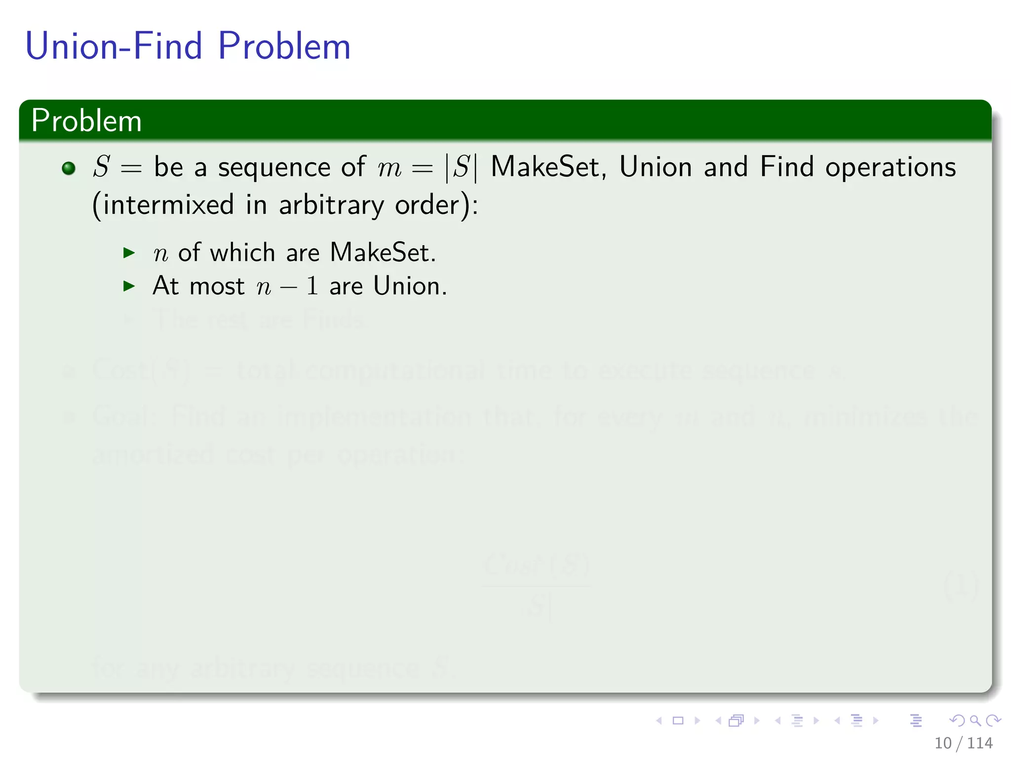


![Circular lists
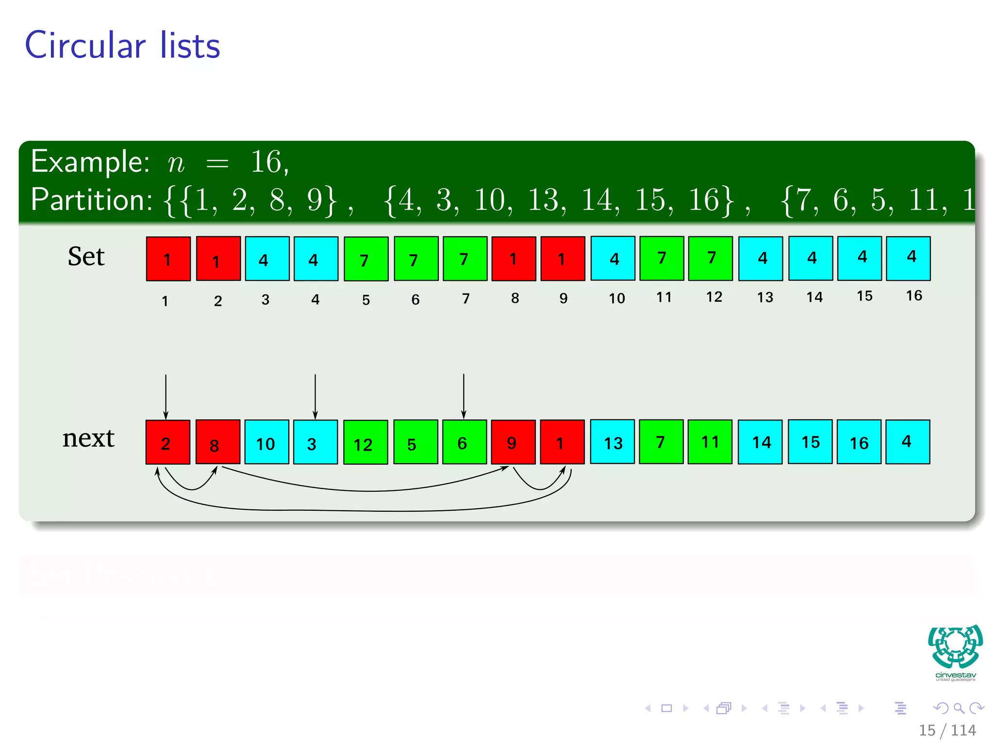
We use the following structures
Data structure: Two arrays Set[1..n] and next[1..n].
Set[x] returns the name of the set that contains item x.
A is a set if and only if Set[A] = A
next[x] returns the next item on the list of the set that contains item
x.
14 / 114](https://image.slidesharecdn.com/17disjointsetrepresentation-151108151359-lva1-app6892/75/17-Disjoint-Set-Representation-33-2048.jpg)
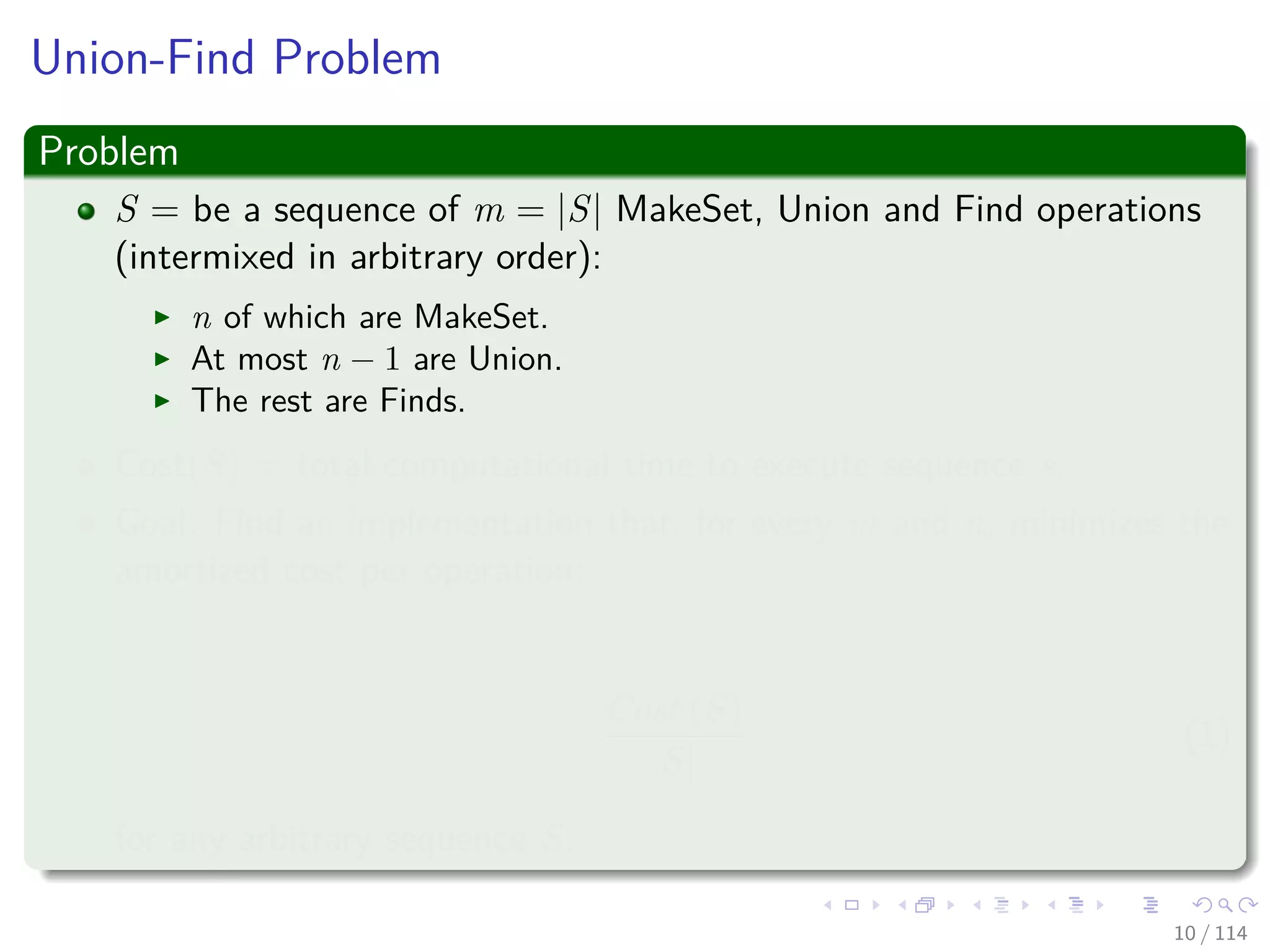
![Circular lists
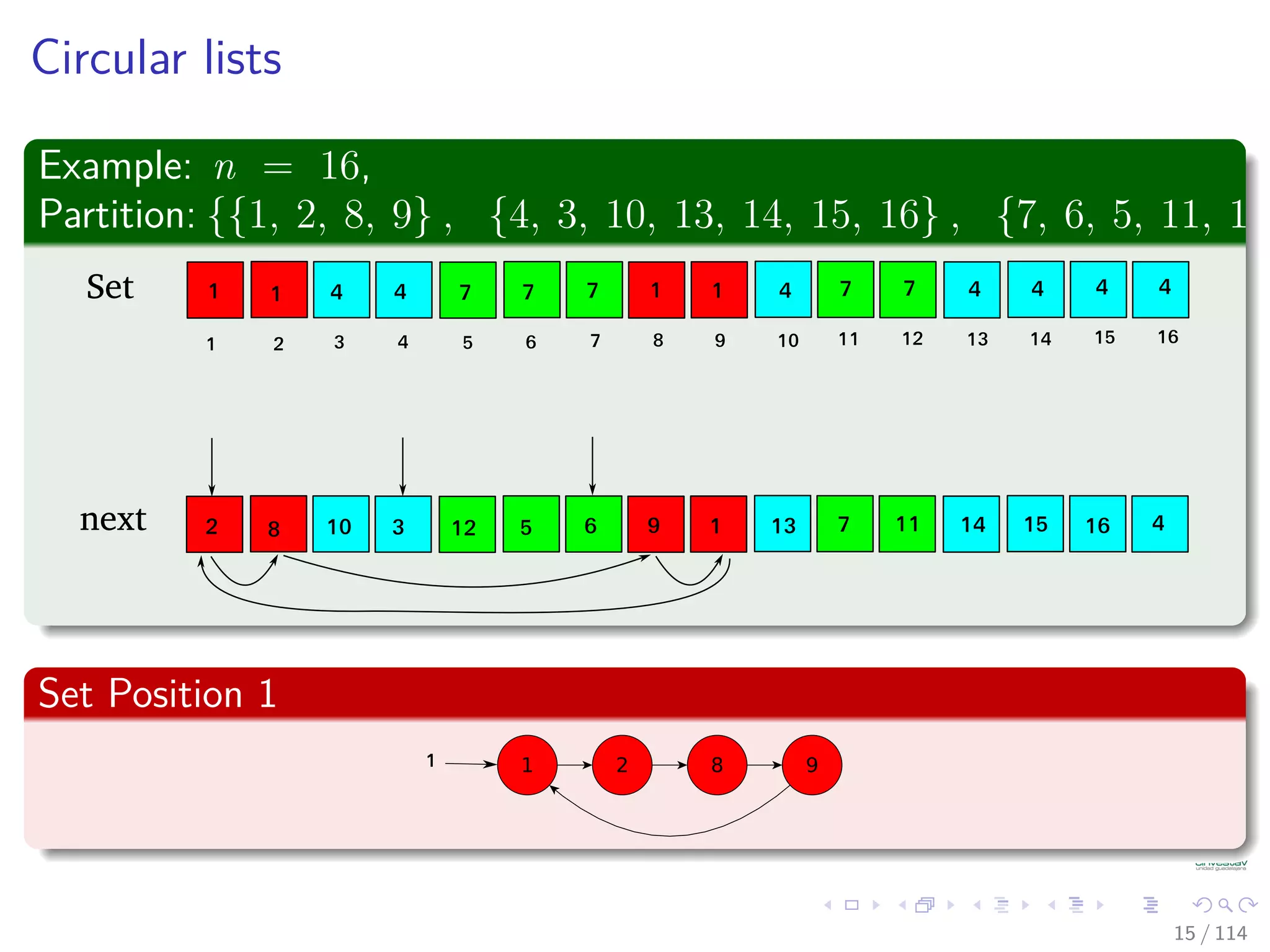
We use the following structures
Data structure: Two arrays Set[1..n] and next[1..n].
Set[x] returns the name of the set that contains item x.
A is a set if and only if Set[A] = A
next[x] returns the next item on the list of the set that contains item
x.
14 / 114](https://image.slidesharecdn.com/17disjointsetrepresentation-151108151359-lva1-app6892/75/17-Disjoint-Set-Representation-34-2048.jpg)
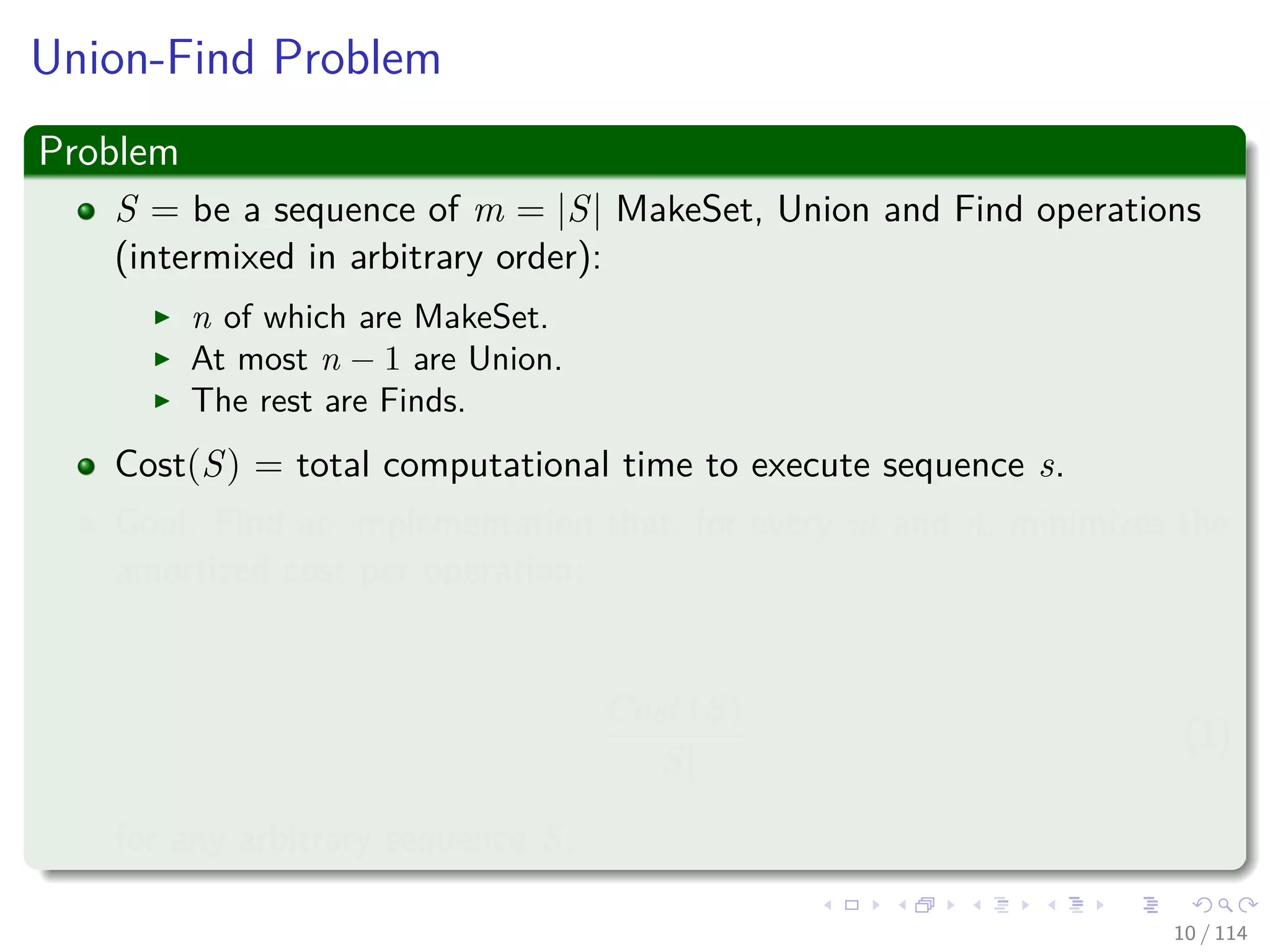
![Circular lists
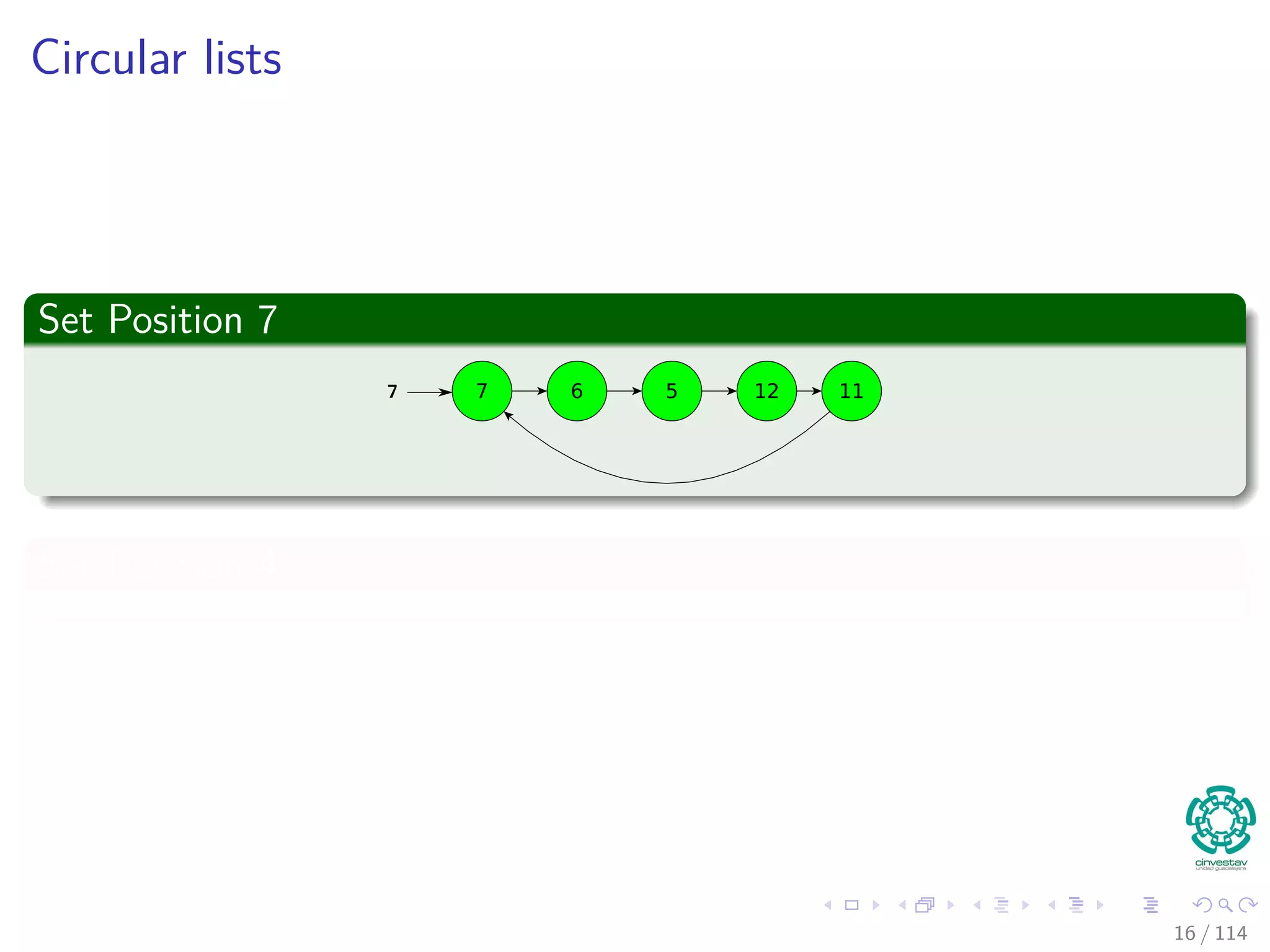
We use the following structures
Data structure: Two arrays Set[1..n] and next[1..n].
Set[x] returns the name of the set that contains item x.
A is a set if and only if Set[A] = A
next[x] returns the next item on the list of the set that contains item
x.
14 / 114](https://image.slidesharecdn.com/17disjointsetrepresentation-151108151359-lva1-app6892/75/17-Disjoint-Set-Representation-35-2048.jpg)
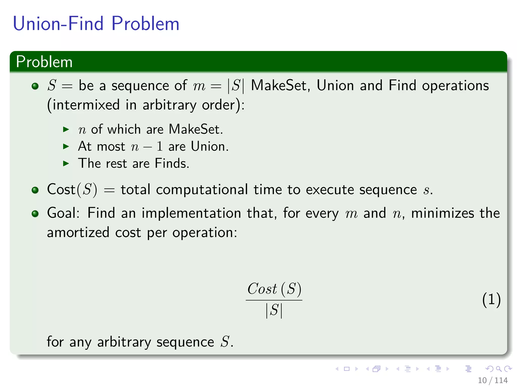
![Circular lists
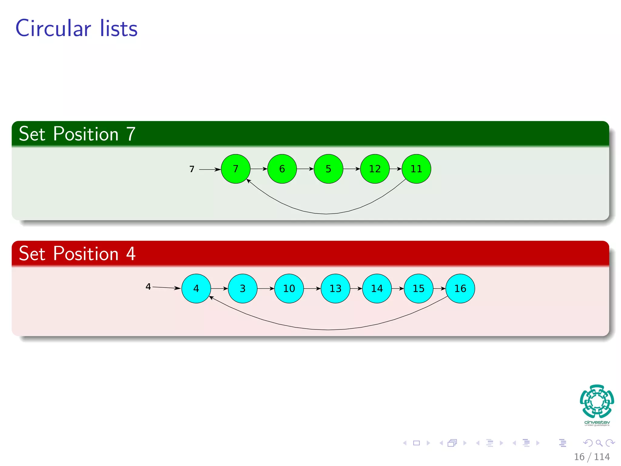
We use the following structures
Data structure: Two arrays Set[1..n] and next[1..n].
Set[x] returns the name of the set that contains item x.
A is a set if and only if Set[A] = A
next[x] returns the next item on the list of the set that contains item
x.
14 / 114](https://image.slidesharecdn.com/17disjointsetrepresentation-151108151359-lva1-app6892/75/17-Disjoint-Set-Representation-36-2048.jpg)
![Operations and Cost
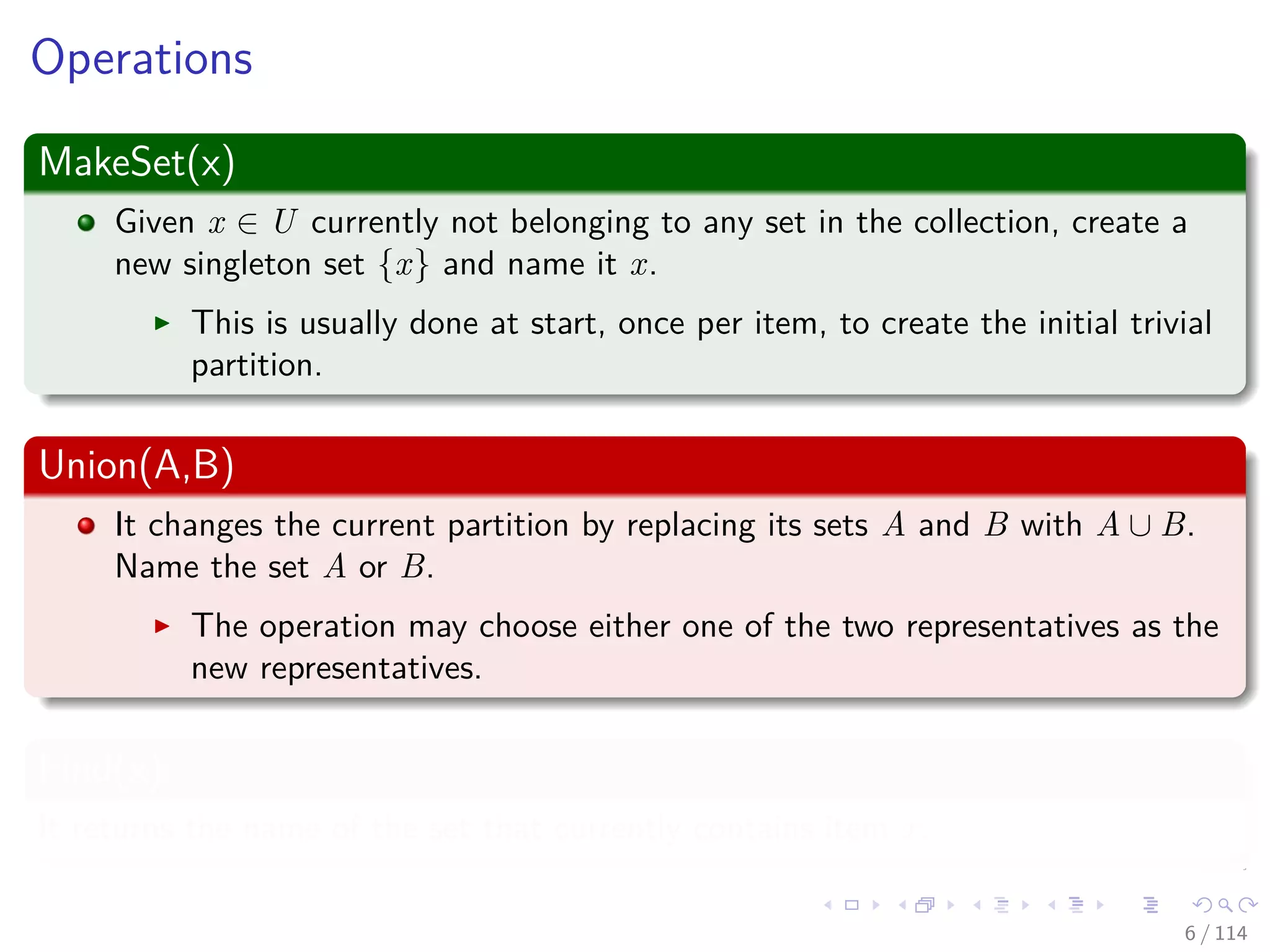
Make(x)
1 Set[x] = x
2 next[x] = x
Complexity
O (1) Time
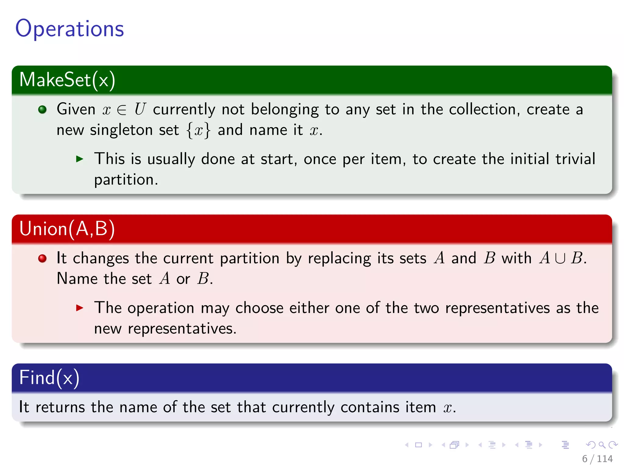
Find(x)
1 return Set[x]
Complexity
O (1) Time
17 / 114](https://image.slidesharecdn.com/17disjointsetrepresentation-151108151359-lva1-app6892/75/17-Disjoint-Set-Representation-41-2048.jpg)
![Operations and Cost
Make(x)
1 Set[x] = x
2 next[x] = x
Complexity
O (1) Time
Find(x)
1 return Set[x]
Complexity
O (1) Time
17 / 114](https://image.slidesharecdn.com/17disjointsetrepresentation-151108151359-lva1-app6892/75/17-Disjoint-Set-Representation-42-2048.jpg)
![Operations and Cost
Make(x)
1 Set[x] = x
2 next[x] = x
Complexity
O (1) Time
Find(x)
1 return Set[x]
Complexity
O (1) Time
17 / 114](https://image.slidesharecdn.com/17disjointsetrepresentation-151108151359-lva1-app6892/75/17-Disjoint-Set-Representation-43-2048.jpg)
![Operations and Cost
Make(x)
1 Set[x] = x
2 next[x] = x
Complexity
O (1) Time
Find(x)
1 return Set[x]
Complexity
O (1) Time
17 / 114](https://image.slidesharecdn.com/17disjointsetrepresentation-151108151359-lva1-app6892/75/17-Disjoint-Set-Representation-44-2048.jpg)
![Operations and Cost
For the union
We are assuming Set[A] = A =Set[B] = B
Union1(A, B)
1 Set[B] = A
2 x =next[B]
3 while (x = B)
4 Set[x] = A /* Rename Set B to A*/
5 x =next[x]
6 x =next[B] /* Splice list A and B */
7 next[B] =next[A]
8 next[A] = x
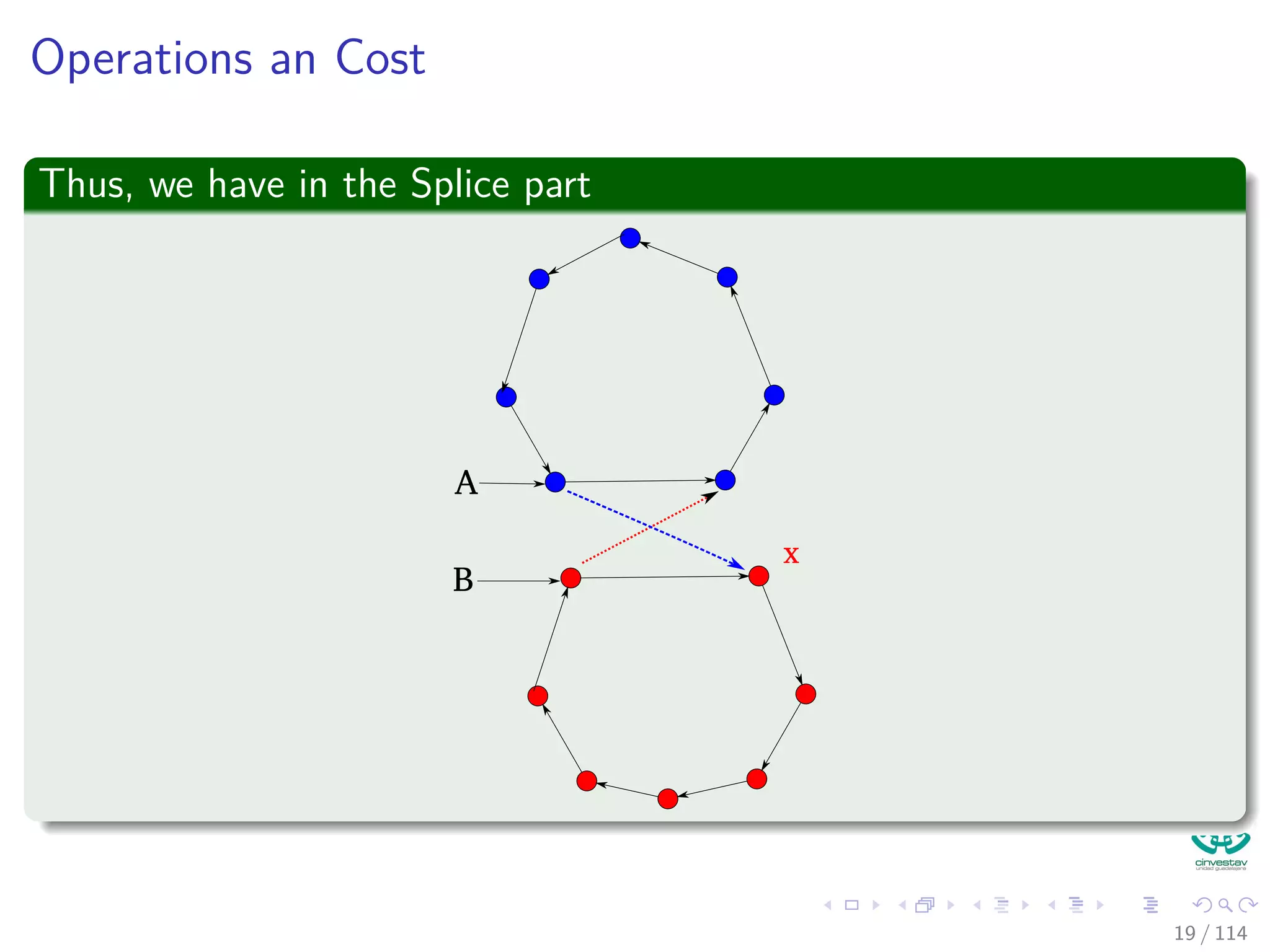
18 / 114](https://image.slidesharecdn.com/17disjointsetrepresentation-151108151359-lva1-app6892/75/17-Disjoint-Set-Representation-45-2048.jpg)
![Operations and Cost
For the union
We are assuming Set[A] = A =Set[B] = B
Union1(A, B)
1 Set[B] = A
2 x =next[B]
3 while (x = B)
4 Set[x] = A /* Rename Set B to A*/
5 x =next[x]
6 x =next[B] /* Splice list A and B */
7 next[B] =next[A]
8 next[A] = x
18 / 114](https://image.slidesharecdn.com/17disjointsetrepresentation-151108151359-lva1-app6892/75/17-Disjoint-Set-Representation-46-2048.jpg)
![Operations and Cost
For the union
We are assuming Set[A] = A =Set[B] = B
Union1(A, B)
1 Set[B] = A
2 x =next[B]
3 while (x = B)
4 Set[x] = A /* Rename Set B to A*/
5 x =next[x]
6 x =next[B] /* Splice list A and B */
7 next[B] =next[A]
8 next[A] = x
18 / 114](https://image.slidesharecdn.com/17disjointsetrepresentation-151108151359-lva1-app6892/75/17-Disjoint-Set-Representation-47-2048.jpg)


![Implementation 2: Weighted-Union Heuristic Lists
We extend the previous data structure
Data structure: Three arrays Set[1..n], next[1..n], size[1..n].
size[A] returns the number of items in set A if A == Set[A]
(Otherwise, we do not care).
25 / 114](https://image.slidesharecdn.com/17disjointsetrepresentation-151108151359-lva1-app6892/75/17-Disjoint-Set-Representation-60-2048.jpg)
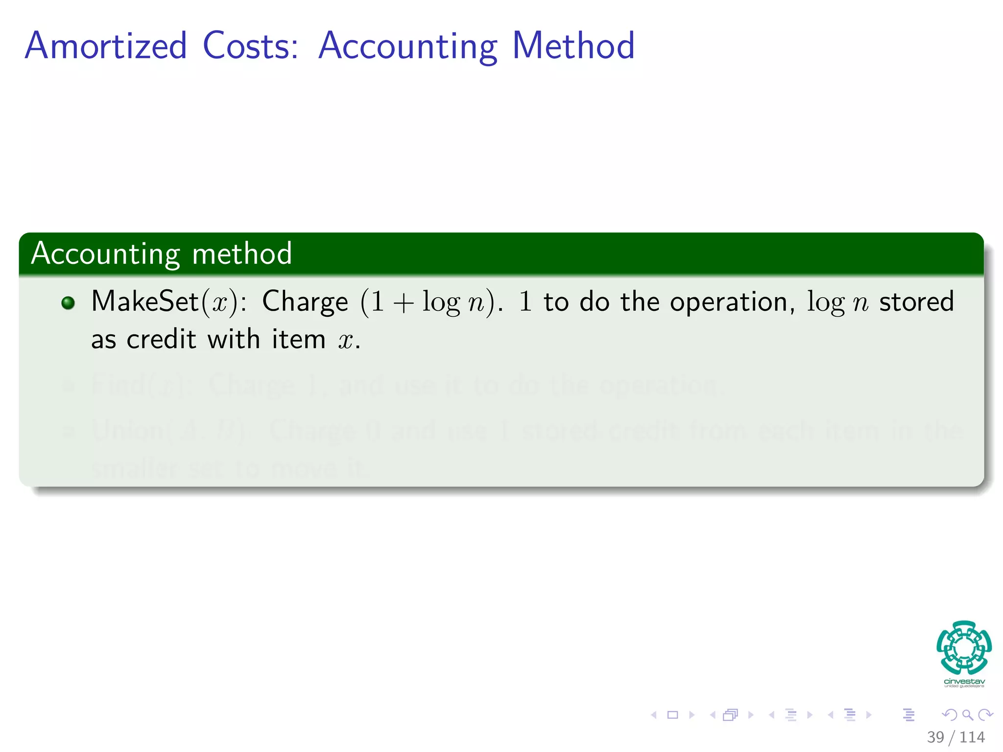
![Operations
MakeSet(x)
1 Set[x] = x
2 next[x] = x
3 size[x] = 1
Complexity
O (1) time
Find(x)
1 return Set[x]
Complexity
O (1) time
26 / 114](https://image.slidesharecdn.com/17disjointsetrepresentation-151108151359-lva1-app6892/75/17-Disjoint-Set-Representation-61-2048.jpg)
![Operations
MakeSet(x)
1 Set[x] = x
2 next[x] = x
3 size[x] = 1
Complexity
O (1) time
Find(x)
1 return Set[x]
Complexity
O (1) time
26 / 114](https://image.slidesharecdn.com/17disjointsetrepresentation-151108151359-lva1-app6892/75/17-Disjoint-Set-Representation-62-2048.jpg)
![Operations
MakeSet(x)
1 Set[x] = x
2 next[x] = x
3 size[x] = 1
Complexity
O (1) time
Find(x)
1 return Set[x]
Complexity
O (1) time
26 / 114](https://image.slidesharecdn.com/17disjointsetrepresentation-151108151359-lva1-app6892/75/17-Disjoint-Set-Representation-63-2048.jpg)
![Operations
MakeSet(x)
1 Set[x] = x
2 next[x] = x
3 size[x] = 1
Complexity
O (1) time
Find(x)
1 return Set[x]
Complexity
O (1) time
26 / 114](https://image.slidesharecdn.com/17disjointsetrepresentation-151108151359-lva1-app6892/75/17-Disjoint-Set-Representation-64-2048.jpg)
![Operations
Union2(A, B)
1 if size[set [A]] >size[set [B]]
2 size[set [A]] =size[set [A]]+size[set [B]]
3 Union1(A, B)
4 else
5 size[set [B]] =size[set [A]]+size[set [B]]
6 Union1(B, A)
Note: Weight Balanced Union: Merge smaller set into large set
Complexity
O (min {|A| , |B|}) time.
27 / 114](https://image.slidesharecdn.com/17disjointsetrepresentation-151108151359-lva1-app6892/75/17-Disjoint-Set-Representation-65-2048.jpg)
![Operations
Union2(A, B)
1 if size[set [A]] >size[set [B]]
2 size[set [A]] =size[set [A]]+size[set [B]]
3 Union1(A, B)
4 else
5 size[set [B]] =size[set [A]]+size[set [B]]
6 Union1(B, A)
Note: Weight Balanced Union: Merge smaller set into large set
Complexity
O (min {|A| , |B|}) time.
27 / 114](https://image.slidesharecdn.com/17disjointsetrepresentation-151108151359-lva1-app6892/75/17-Disjoint-Set-Representation-66-2048.jpg)


![Improving over the heuristic using union by rank
Union by Rank
Instead of using the number of nodes in each tree to make a decision, we
maintain a rank, a upper bound on the height of the tree.
We have the following data structure to support this:
We maintain a parent array p[1..n].
A is a set if and only if A = p[A] (a tree root).
x ∈ A if and only if x is in the tree rooted at A.
43 / 114](https://image.slidesharecdn.com/17disjointsetrepresentation-151108151359-lva1-app6892/75/17-Disjoint-Set-Representation-108-2048.jpg)
![Improving over the heuristic using union by rank
Union by Rank
Instead of using the number of nodes in each tree to make a decision, we
maintain a rank, a upper bound on the height of the tree.
We have the following data structure to support this:
We maintain a parent array p[1..n].
A is a set if and only if A = p[A] (a tree root).
x ∈ A if and only if x is in the tree rooted at A.
43 / 114](https://image.slidesharecdn.com/17disjointsetrepresentation-151108151359-lva1-app6892/75/17-Disjoint-Set-Representation-109-2048.jpg)
![Improving over the heuristic using union by rank
Union by Rank
Instead of using the number of nodes in each tree to make a decision, we
maintain a rank, a upper bound on the height of the tree.
We have the following data structure to support this:
We maintain a parent array p[1..n].
A is a set if and only if A = p[A] (a tree root).
x ∈ A if and only if x is in the tree rooted at A.
43 / 114](https://image.slidesharecdn.com/17disjointsetrepresentation-151108151359-lva1-app6892/75/17-Disjoint-Set-Representation-110-2048.jpg)
![Improving over the heuristic using union by rank
Union by Rank
Instead of using the number of nodes in each tree to make a decision, we
maintain a rank, a upper bound on the height of the tree.
We have the following data structure to support this:
We maintain a parent array p[1..n].
A is a set if and only if A = p[A] (a tree root).
x ∈ A if and only if x is in the tree rooted at A.
43 / 114](https://image.slidesharecdn.com/17disjointsetrepresentation-151108151359-lva1-app6892/75/17-Disjoint-Set-Representation-111-2048.jpg)
![Improving over the heuristic using union by rank
Union by Rank
Instead of using the number of nodes in each tree to make a decision, we
maintain a rank, a upper bound on the height of the tree.
We have the following data structure to support this:
We maintain a parent array p[1..n].
A is a set if and only if A = p[A] (a tree root).
x ∈ A if and only if x is in the tree rooted at A.
1
13 5 8
20 14 10
19
4
2 18 6
15 9 11
17
7
3
12
16
43 / 114](https://image.slidesharecdn.com/17disjointsetrepresentation-151108151359-lva1-app6892/75/17-Disjoint-Set-Representation-112-2048.jpg)
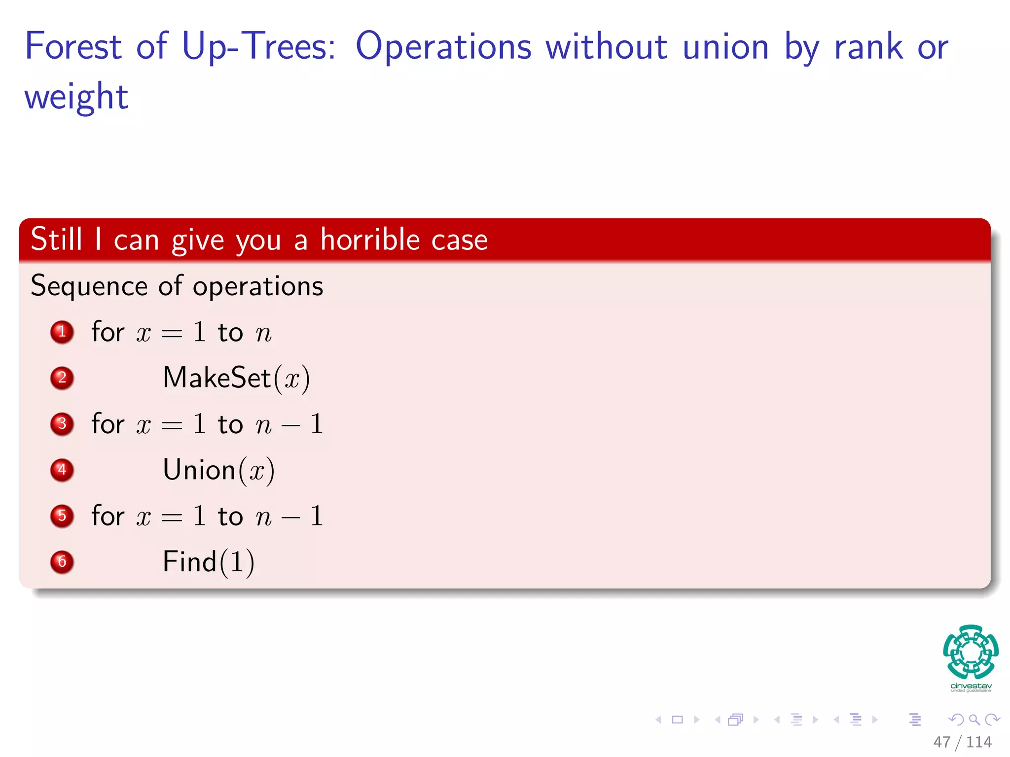
![Forest of Up-Trees: Operations without union by rank or
weight
MakeSet(x)
1 p[x] = x
Complexity
O (1) time
Union(A, B)
1 p[B] = A
Note: We are assuming that p[A] == A =p[B] == B. This is the
reason we need a find operation!!!
44 / 114](https://image.slidesharecdn.com/17disjointsetrepresentation-151108151359-lva1-app6892/75/17-Disjoint-Set-Representation-113-2048.jpg)
![Forest of Up-Trees: Operations without union by rank or
weight
MakeSet(x)
1 p[x] = x
Complexity
O (1) time
Union(A, B)
1 p[B] = A
Note: We are assuming that p[A] == A =p[B] == B. This is the
reason we need a find operation!!!
44 / 114](https://image.slidesharecdn.com/17disjointsetrepresentation-151108151359-lva1-app6892/75/17-Disjoint-Set-Representation-114-2048.jpg)
![Forest of Up-Trees: Operations without union by rank or
weight
MakeSet(x)
1 p[x] = x
Complexity
O (1) time
Union(A, B)
1 p[B] = A
Note: We are assuming that p[A] == A =p[B] == B. This is the
reason we need a find operation!!!
44 / 114](https://image.slidesharecdn.com/17disjointsetrepresentation-151108151359-lva1-app6892/75/17-Disjoint-Set-Representation-115-2048.jpg)
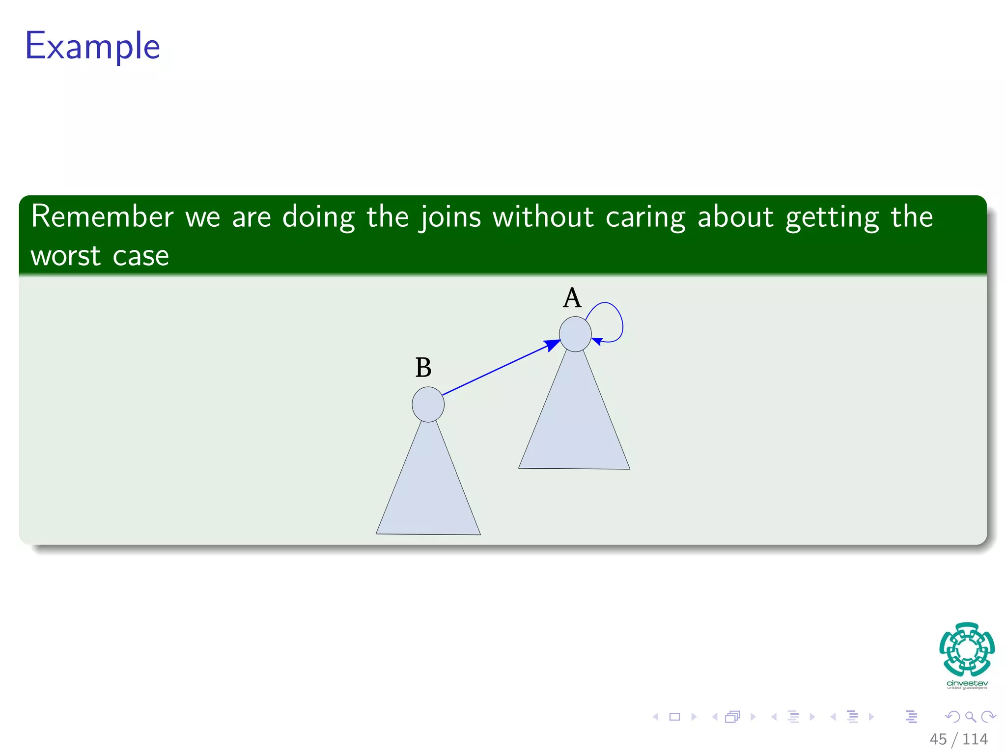
![Forest of Up-Trees: Operations without union by rank or
weight
Find(x)
1 if x ==p[x]
2 return x
3 return Find(p [x])
Example
46 / 114](https://image.slidesharecdn.com/17disjointsetrepresentation-151108151359-lva1-app6892/75/17-Disjoint-Set-Representation-117-2048.jpg)
![Forest of Up-Trees: Operations without union by rank or
weight
Find(x)
1 if x ==p[x]
2 return x
3 return Find(p [x])
Example
x
46 / 114](https://image.slidesharecdn.com/17disjointsetrepresentation-151108151359-lva1-app6892/75/17-Disjoint-Set-Representation-118-2048.jpg)

![We have then
MakeSet(x)
1 p[x] = x
2 size[x] = 1
Note: Complexity O (1) time
Union(A, B)
Input: assume that p[A]=A=p[B]=B
1 if size[A] >size[B]
2 size[A] =size[A]+size[B]
3 p[B] = A
4 else
5 size[B] =size[A]+size[B]
6 p[A] = B
Note: Complexity O (1) time
51 / 114](https://image.slidesharecdn.com/17disjointsetrepresentation-151108151359-lva1-app6892/75/17-Disjoint-Set-Representation-131-2048.jpg)
![We have then
MakeSet(x)
1 p[x] = x
2 size[x] = 1
Note: Complexity O (1) time
Union(A, B)
Input: assume that p[A]=A=p[B]=B
1 if size[A] >size[B]
2 size[A] =size[A]+size[B]
3 p[B] = A
4 else
5 size[B] =size[A]+size[B]
6 p[A] = B
Note: Complexity O (1) time
51 / 114](https://image.slidesharecdn.com/17disjointsetrepresentation-151108151359-lva1-app6892/75/17-Disjoint-Set-Representation-132-2048.jpg)
![We have then
MakeSet(x)
1 p[x] = x
2 size[x] = 1
Note: Complexity O (1) time
Union(A, B)
Input: assume that p[A]=A=p[B]=B
1 if size[A] >size[B]
2 size[A] =size[A]+size[B]
3 p[B] = A
4 else
5 size[B] =size[A]+size[B]
6 p[A] = B
Note: Complexity O (1) time
51 / 114](https://image.slidesharecdn.com/17disjointsetrepresentation-151108151359-lva1-app6892/75/17-Disjoint-Set-Representation-133-2048.jpg)
![Example
Now, we use the size for the union
size[A]>size[B]
B
A
52 / 114](https://image.slidesharecdn.com/17disjointsetrepresentation-151108151359-lva1-app6892/75/17-Disjoint-Set-Representation-134-2048.jpg)

![Thus, we use the balanced union by rank
MakeSet(x)
1 p[x] = x
2 rank[x] = 0
Note: Complexity O (1) time
Union(A, B)
Input: assume that p[A]=A=p[B]=B
1 if rank[A] >rank[B]
2 p[B] = A
3 else
4 p[A] = B
5 if rank[A] ==rank[B]
6 rank[B]=rank[B]+1
Note: Complexity O (1) time
54 / 114](https://image.slidesharecdn.com/17disjointsetrepresentation-151108151359-lva1-app6892/75/17-Disjoint-Set-Representation-138-2048.jpg)
![Thus, we use the balanced union by rank
MakeSet(x)
1 p[x] = x
2 rank[x] = 0
Note: Complexity O (1) time
Union(A, B)
Input: assume that p[A]=A=p[B]=B
1 if rank[A] >rank[B]
2 p[B] = A
3 else
4 p[A] = B
5 if rank[A] ==rank[B]
6 rank[B]=rank[B]+1
Note: Complexity O (1) time
54 / 114](https://image.slidesharecdn.com/17disjointsetrepresentation-151108151359-lva1-app6892/75/17-Disjoint-Set-Representation-139-2048.jpg)
![Thus, we use the balanced union by rank
MakeSet(x)
1 p[x] = x
2 rank[x] = 0
Note: Complexity O (1) time
Union(A, B)
Input: assume that p[A]=A=p[B]=B
1 if rank[A] >rank[B]
2 p[B] = A
3 else
4 p[A] = B
5 if rank[A] ==rank[B]
6 rank[B]=rank[B]+1
Note: Complexity O (1) time
54 / 114](https://image.slidesharecdn.com/17disjointsetrepresentation-151108151359-lva1-app6892/75/17-Disjoint-Set-Representation-140-2048.jpg)

![Example
Now
We use the rank for the union
Case I
The rank of A is larger than B
rank[A]>rank[B]
B
A
55 / 114](https://image.slidesharecdn.com/17disjointsetrepresentation-151108151359-lva1-app6892/75/17-Disjoint-Set-Representation-142-2048.jpg)
![Example
Case II
The rank of B is larger than A
rank[B]>rank[A]
B
A
56 / 114](https://image.slidesharecdn.com/17disjointsetrepresentation-151108151359-lva1-app6892/75/17-Disjoint-Set-Representation-144-2048.jpg)

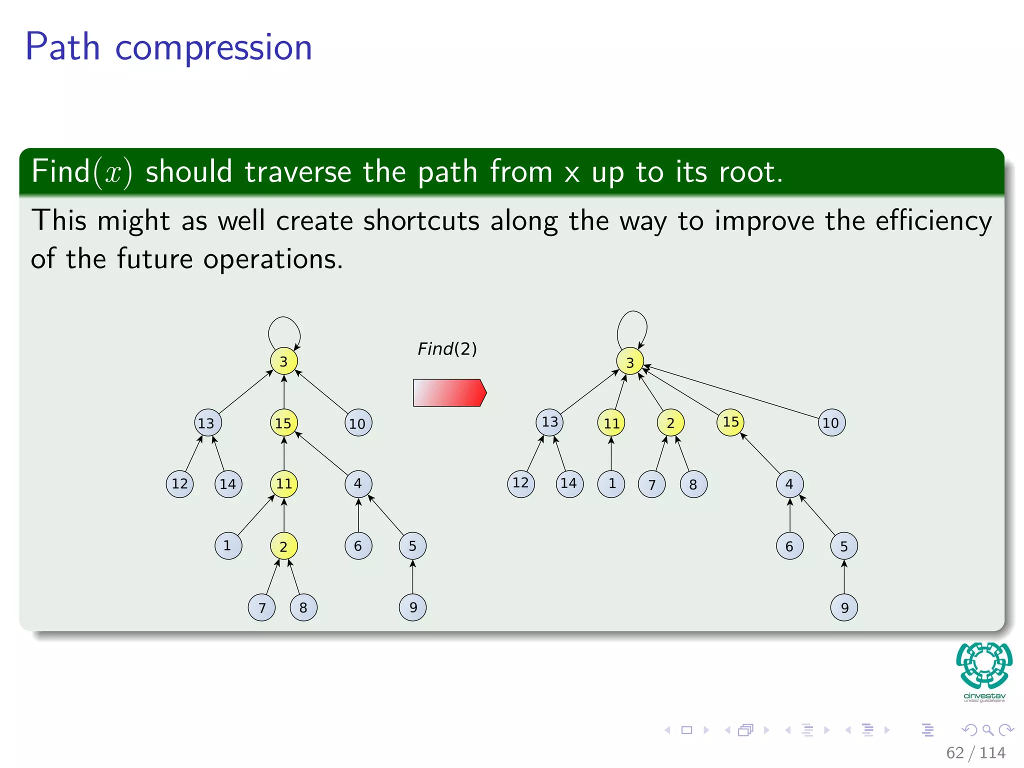
![Here is the new heuristic to improve overall performance:
Path Compression
Find(x)
1 if x=p[x]
2 p[x]=Find(p [x])
3 return p[x]
Complexity
O (depth (x)) time
58 / 114](https://image.slidesharecdn.com/17disjointsetrepresentation-151108151359-lva1-app6892/75/17-Disjoint-Set-Representation-146-2048.jpg)
![Here is the new heuristic to improve overall performance:
Path Compression
Find(x)
1 if x=p[x]
2 p[x]=Find(p [x])
3 return p[x]
Complexity
O (depth (x)) time
58 / 114](https://image.slidesharecdn.com/17disjointsetrepresentation-151108151359-lva1-app6892/75/17-Disjoint-Set-Representation-147-2048.jpg)
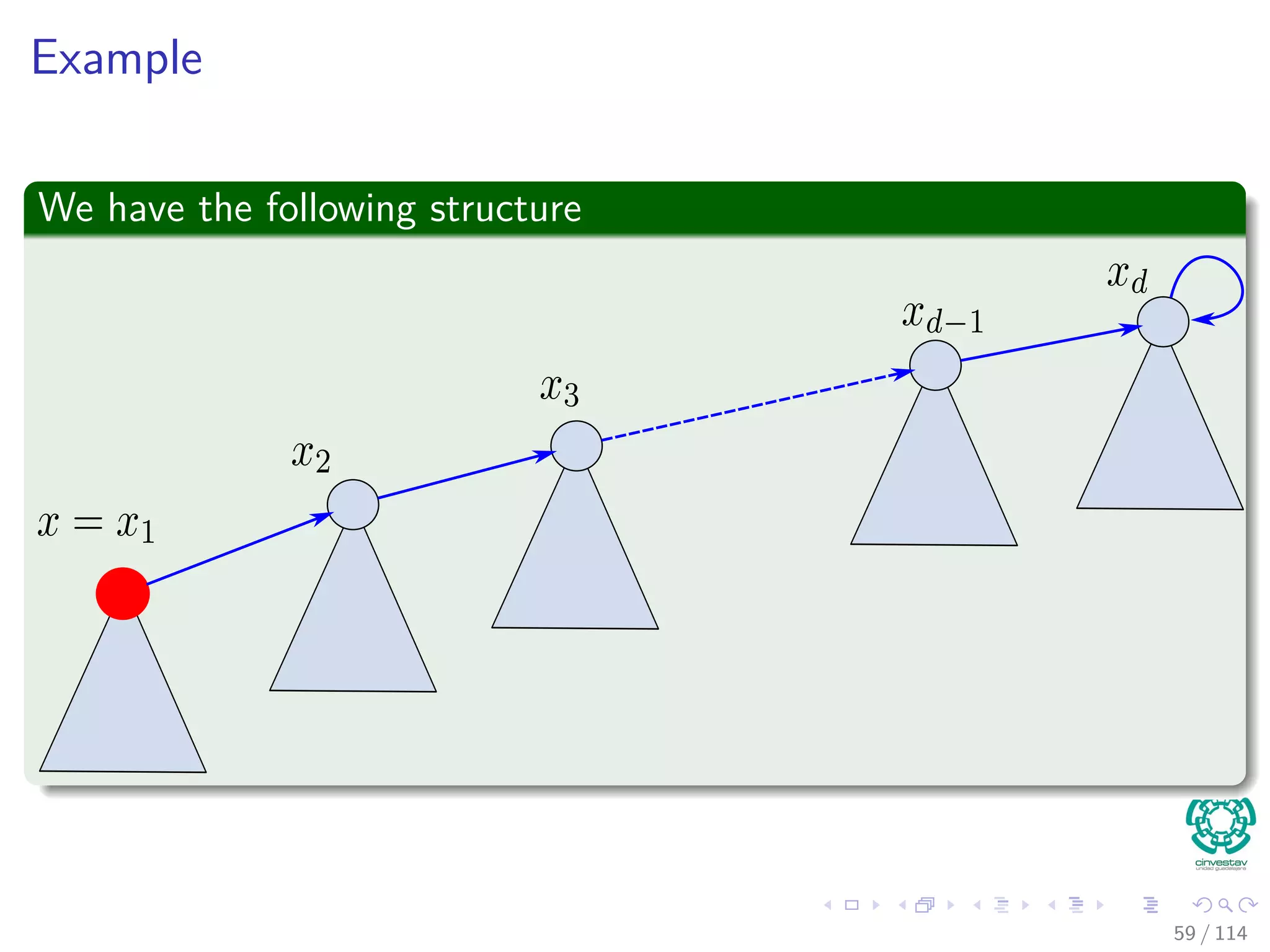
![Example
The recursive Find(p [x])
60 / 114](https://image.slidesharecdn.com/17disjointsetrepresentation-151108151359-lva1-app6892/75/17-Disjoint-Set-Representation-149-2048.jpg)
![Example
The recursive Find(p [x])
61 / 114](https://image.slidesharecdn.com/17disjointsetrepresentation-151108151359-lva1-app6892/75/17-Disjoint-Set-Representation-150-2048.jpg)


![Properties of ranks
Lemma 1 (About the Rank Properties)
1 ∀x, rank[x] ≤ rank[p[x]].
2 ∀x and x = p[x], then rank[x] < rank[p[x]].
3 rank[x] is initially 0.
4 rank[x] does not decrease.
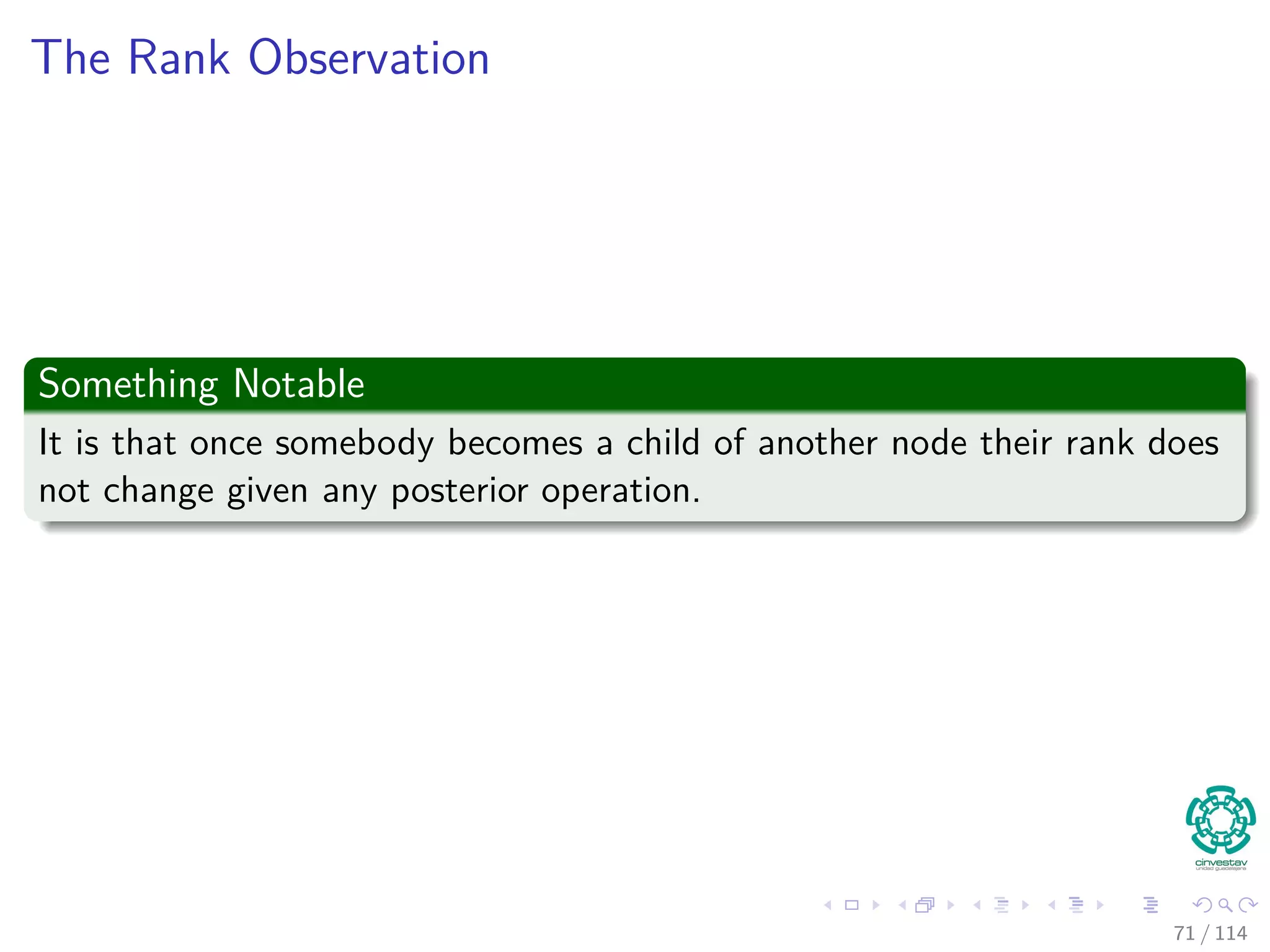
5 Once x = p[x] holds rank[x] does not change.
6 rank[p[x]] is a monotonically increasing function of time.
Proof
By induction on the number of operations...
79 / 114](https://image.slidesharecdn.com/17disjointsetrepresentation-151108151359-lva1-app6892/75/17-Disjoint-Set-Representation-185-2048.jpg)
![Properties of ranks
Lemma 1 (About the Rank Properties)
1 ∀x, rank[x] ≤ rank[p[x]].
2 ∀x and x = p[x], then rank[x] < rank[p[x]].
3 rank[x] is initially 0.
4 rank[x] does not decrease.
5 Once x = p[x] holds rank[x] does not change.
6 rank[p[x]] is a monotonically increasing function of time.
Proof
By induction on the number of operations...
79 / 114](https://image.slidesharecdn.com/17disjointsetrepresentation-151108151359-lva1-app6892/75/17-Disjoint-Set-Representation-186-2048.jpg)
![Properties of ranks
Lemma 1 (About the Rank Properties)
1 ∀x, rank[x] ≤ rank[p[x]].
2 ∀x and x = p[x], then rank[x] < rank[p[x]].
3 rank[x] is initially 0.
4 rank[x] does not decrease.
5 Once x = p[x] holds rank[x] does not change.
6 rank[p[x]] is a monotonically increasing function of time.
Proof
By induction on the number of operations...
79 / 114](https://image.slidesharecdn.com/17disjointsetrepresentation-151108151359-lva1-app6892/75/17-Disjoint-Set-Representation-187-2048.jpg)
![Properties of ranks
Lemma 1 (About the Rank Properties)
1 ∀x, rank[x] ≤ rank[p[x]].
2 ∀x and x = p[x], then rank[x] < rank[p[x]].
3 rank[x] is initially 0.
4 rank[x] does not decrease.
5 Once x = p[x] holds rank[x] does not change.
6 rank[p[x]] is a monotonically increasing function of time.
Proof
By induction on the number of operations...
79 / 114](https://image.slidesharecdn.com/17disjointsetrepresentation-151108151359-lva1-app6892/75/17-Disjoint-Set-Representation-188-2048.jpg)
![Properties of ranks
Lemma 1 (About the Rank Properties)
1 ∀x, rank[x] ≤ rank[p[x]].
2 ∀x and x = p[x], then rank[x] < rank[p[x]].
3 rank[x] is initially 0.
4 rank[x] does not decrease.
5 Once x = p[x] holds rank[x] does not change.
6 rank[p[x]] is a monotonically increasing function of time.
Proof
By induction on the number of operations...
79 / 114](https://image.slidesharecdn.com/17disjointsetrepresentation-151108151359-lva1-app6892/75/17-Disjoint-Set-Representation-189-2048.jpg)
![Properties of ranks
Lemma 1 (About the Rank Properties)
1 ∀x, rank[x] ≤ rank[p[x]].
2 ∀x and x = p[x], then rank[x] < rank[p[x]].
3 rank[x] is initially 0.
4 rank[x] does not decrease.
5 Once x = p[x] holds rank[x] does not change.
6 rank[p[x]] is a monotonically increasing function of time.
Proof
By induction on the number of operations...
79 / 114](https://image.slidesharecdn.com/17disjointsetrepresentation-151108151359-lva1-app6892/75/17-Disjoint-Set-Representation-190-2048.jpg)
![Properties of ranks
Lemma 1 (About the Rank Properties)
1 ∀x, rank[x] ≤ rank[p[x]].
2 ∀x and x = p[x], then rank[x] < rank[p[x]].
3 rank[x] is initially 0.
4 rank[x] does not decrease.
5 Once x = p[x] holds rank[x] does not change.
6 rank[p[x]] is a monotonically increasing function of time.
Proof
By induction on the number of operations...
79 / 114](https://image.slidesharecdn.com/17disjointsetrepresentation-151108151359-lva1-app6892/75/17-Disjoint-Set-Representation-191-2048.jpg)
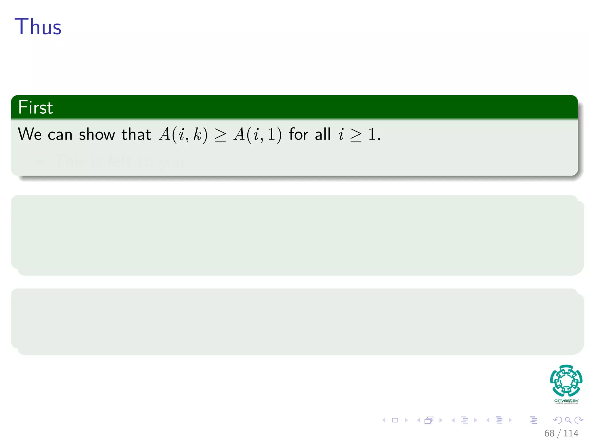
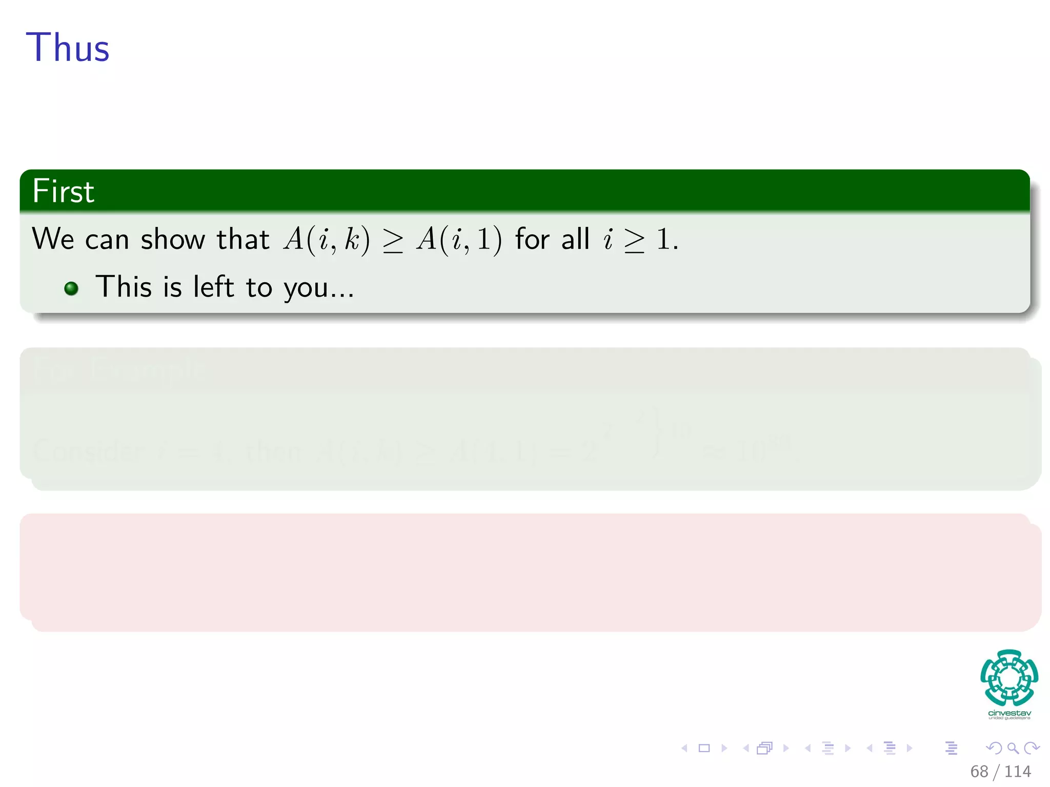
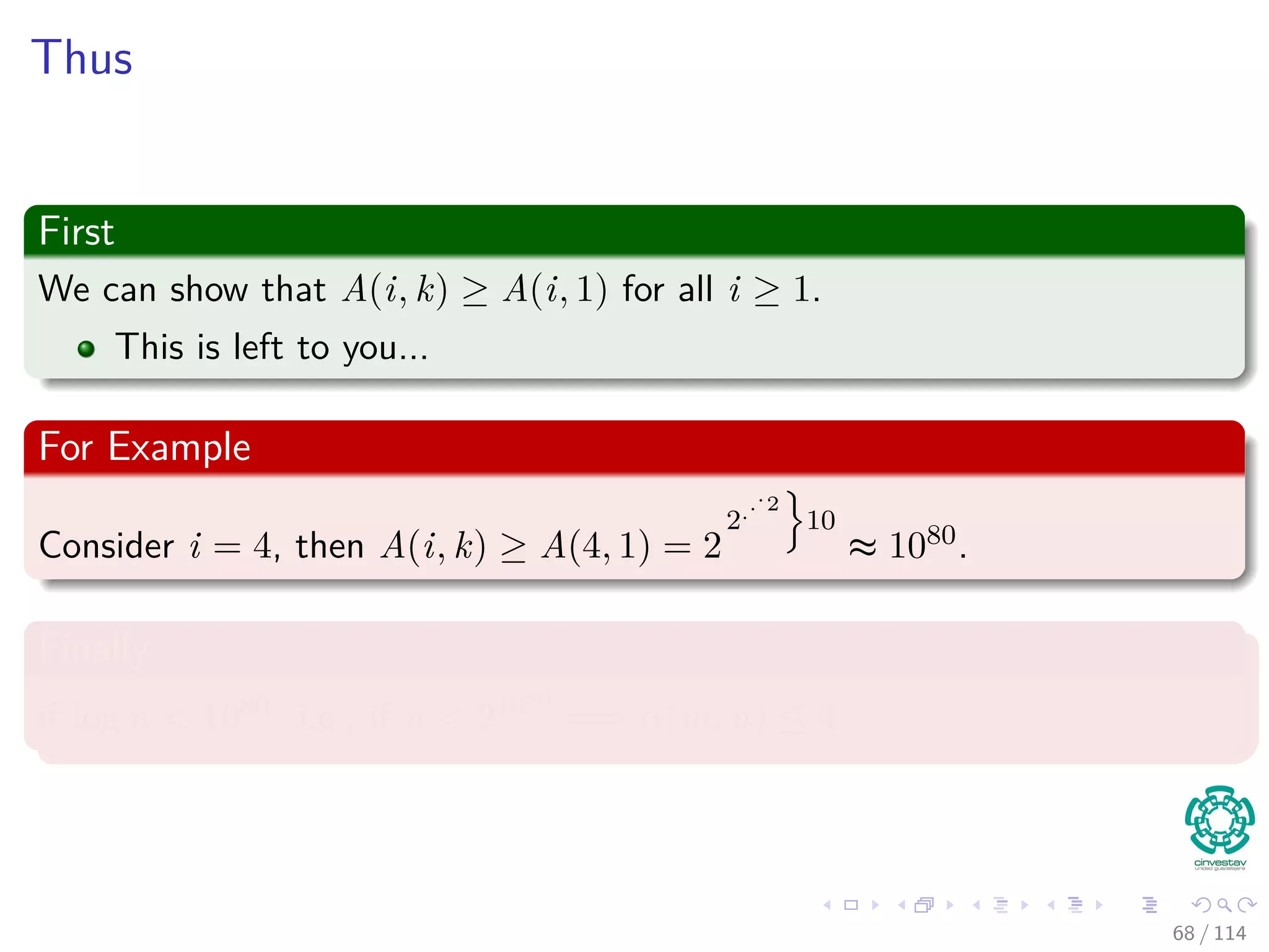
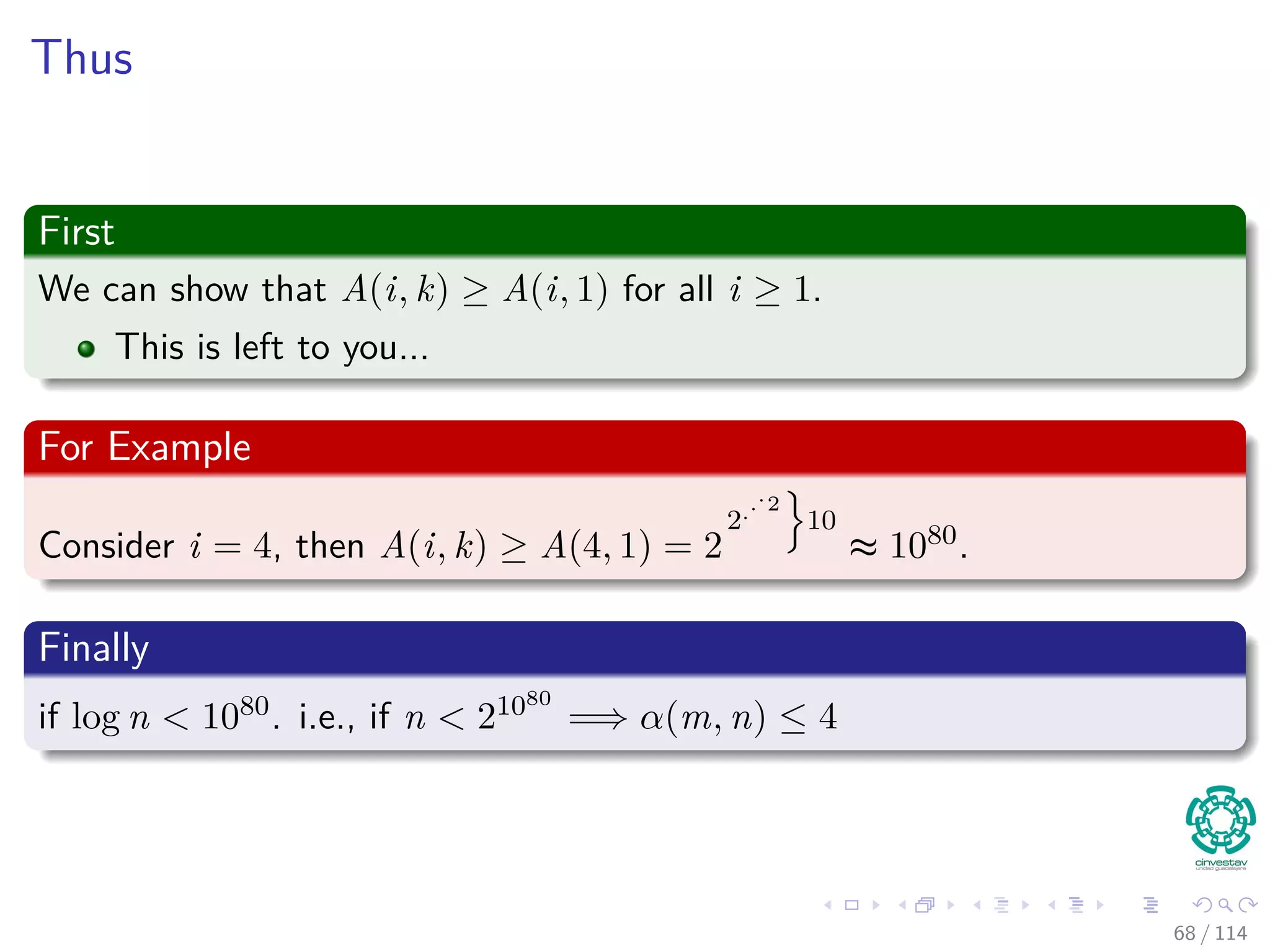
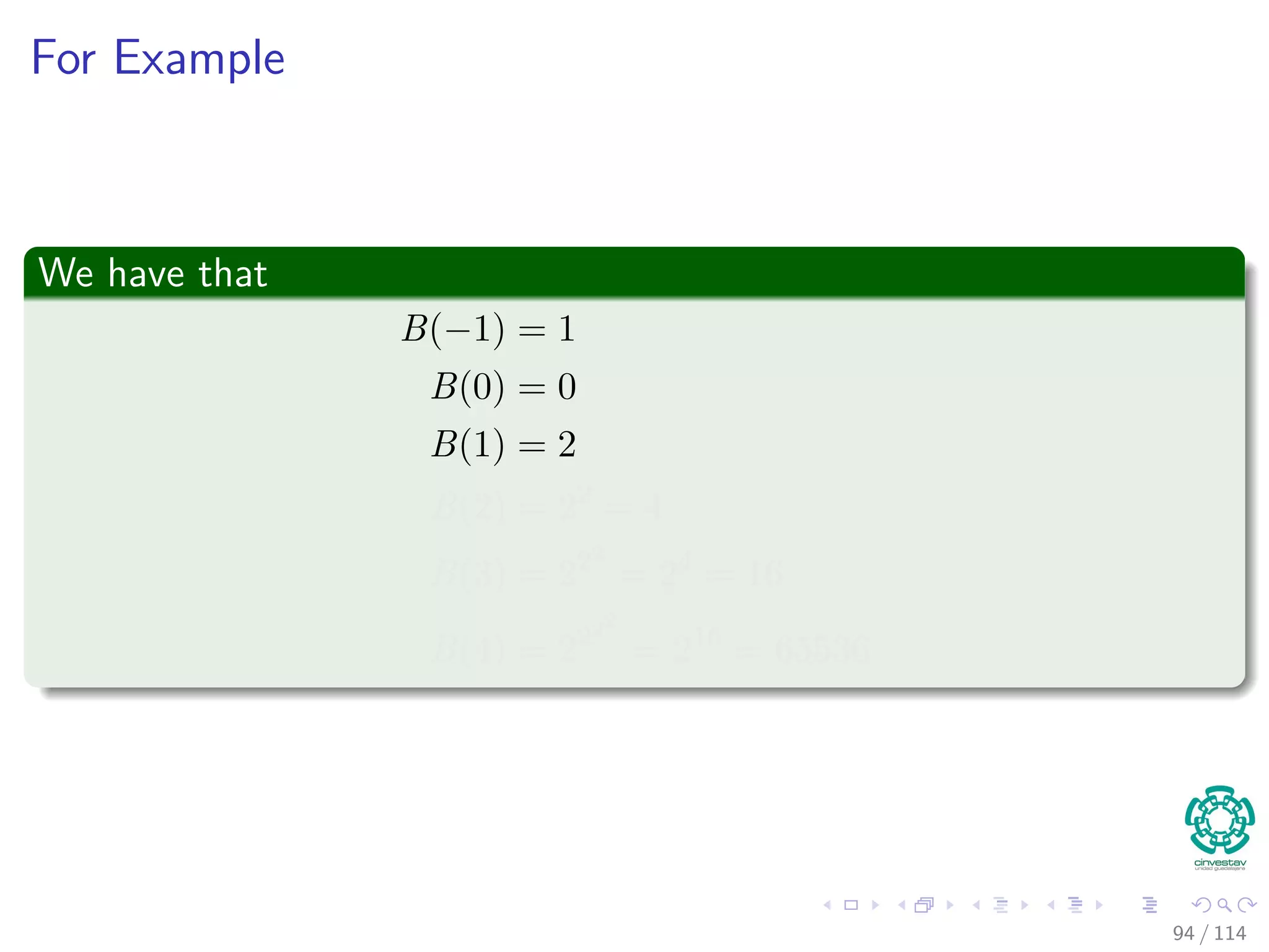
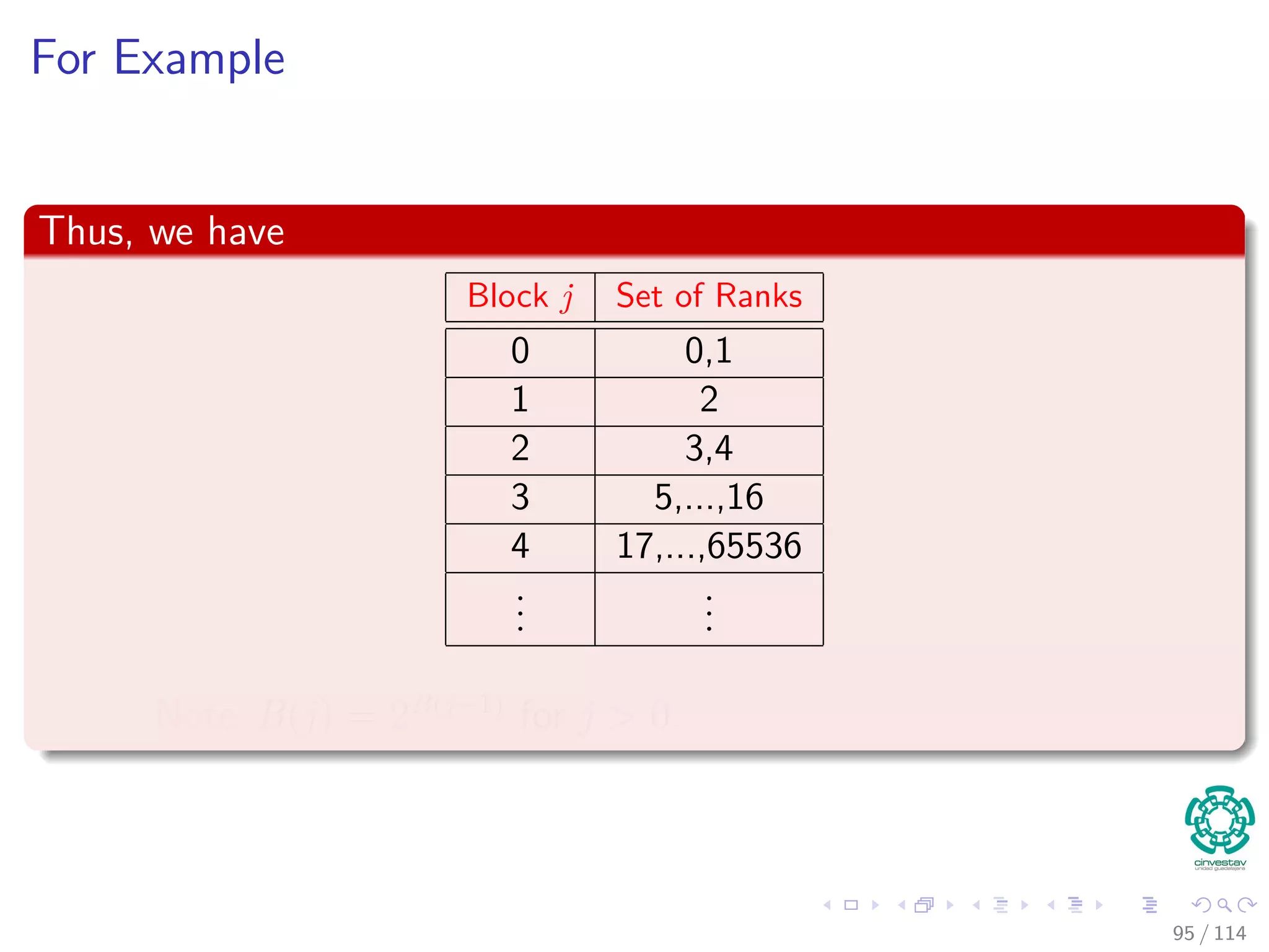
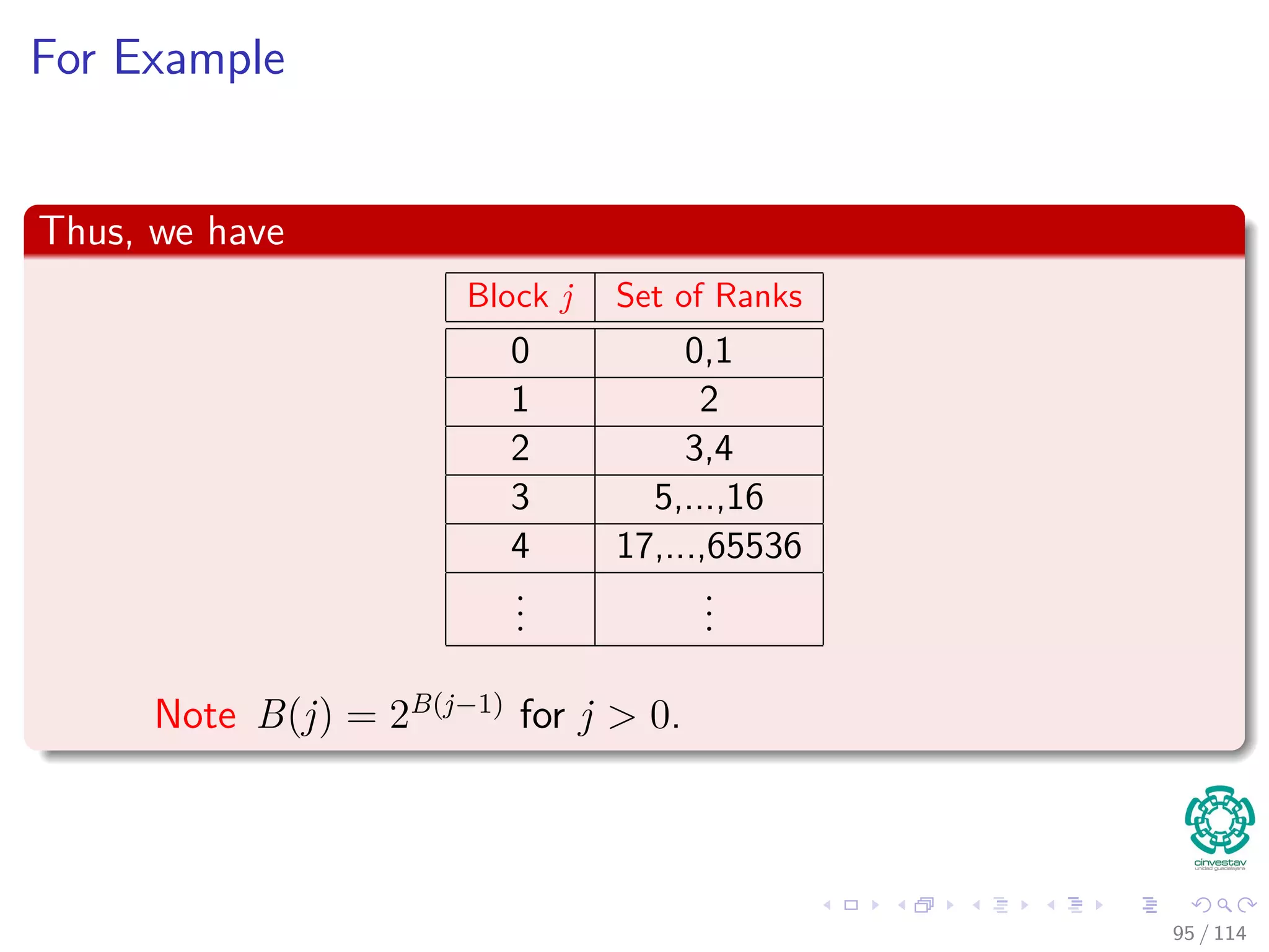
![For Example
Imagine a MakeSet(x)
Then, rank [x] ≤ rank [p [x]]
Thus, it is true after n operations.
The we get the n + 1 operations that can be:
Case I - FindSet.
Case II - Union.
The rest are for you to prove
It is a good mental exercise!!!
80 / 114](https://image.slidesharecdn.com/17disjointsetrepresentation-151108151359-lva1-app6892/75/17-Disjoint-Set-Representation-192-2048.jpg)
![For Example
Imagine a MakeSet(x)
Then, rank [x] ≤ rank [p [x]]
Thus, it is true after n operations.
The we get the n + 1 operations that can be:
Case I - FindSet.
Case II - Union.
The rest are for you to prove
It is a good mental exercise!!!
80 / 114](https://image.slidesharecdn.com/17disjointsetrepresentation-151108151359-lva1-app6892/75/17-Disjoint-Set-Representation-193-2048.jpg)
![For Example
Imagine a MakeSet(x)
Then, rank [x] ≤ rank [p [x]]
Thus, it is true after n operations.
The we get the n + 1 operations that can be:
Case I - FindSet.
Case II - Union.
The rest are for you to prove
It is a good mental exercise!!!
80 / 114](https://image.slidesharecdn.com/17disjointsetrepresentation-151108151359-lva1-app6892/75/17-Disjoint-Set-Representation-194-2048.jpg)
![For Example
Imagine a MakeSet(x)
Then, rank [x] ≤ rank [p [x]]
Thus, it is true after n operations.
The we get the n + 1 operations that can be:
Case I - FindSet.
Case II - Union.
The rest are for you to prove
It is a good mental exercise!!!
80 / 114](https://image.slidesharecdn.com/17disjointsetrepresentation-151108151359-lva1-app6892/75/17-Disjoint-Set-Representation-195-2048.jpg)
![For Example
Imagine a MakeSet(x)
Then, rank [x] ≤ rank [p [x]]
Thus, it is true after n operations.
The we get the n + 1 operations that can be:
Case I - FindSet.
Case II - Union.
The rest are for you to prove
It is a good mental exercise!!!
80 / 114](https://image.slidesharecdn.com/17disjointsetrepresentation-151108151359-lva1-app6892/75/17-Disjoint-Set-Representation-196-2048.jpg)
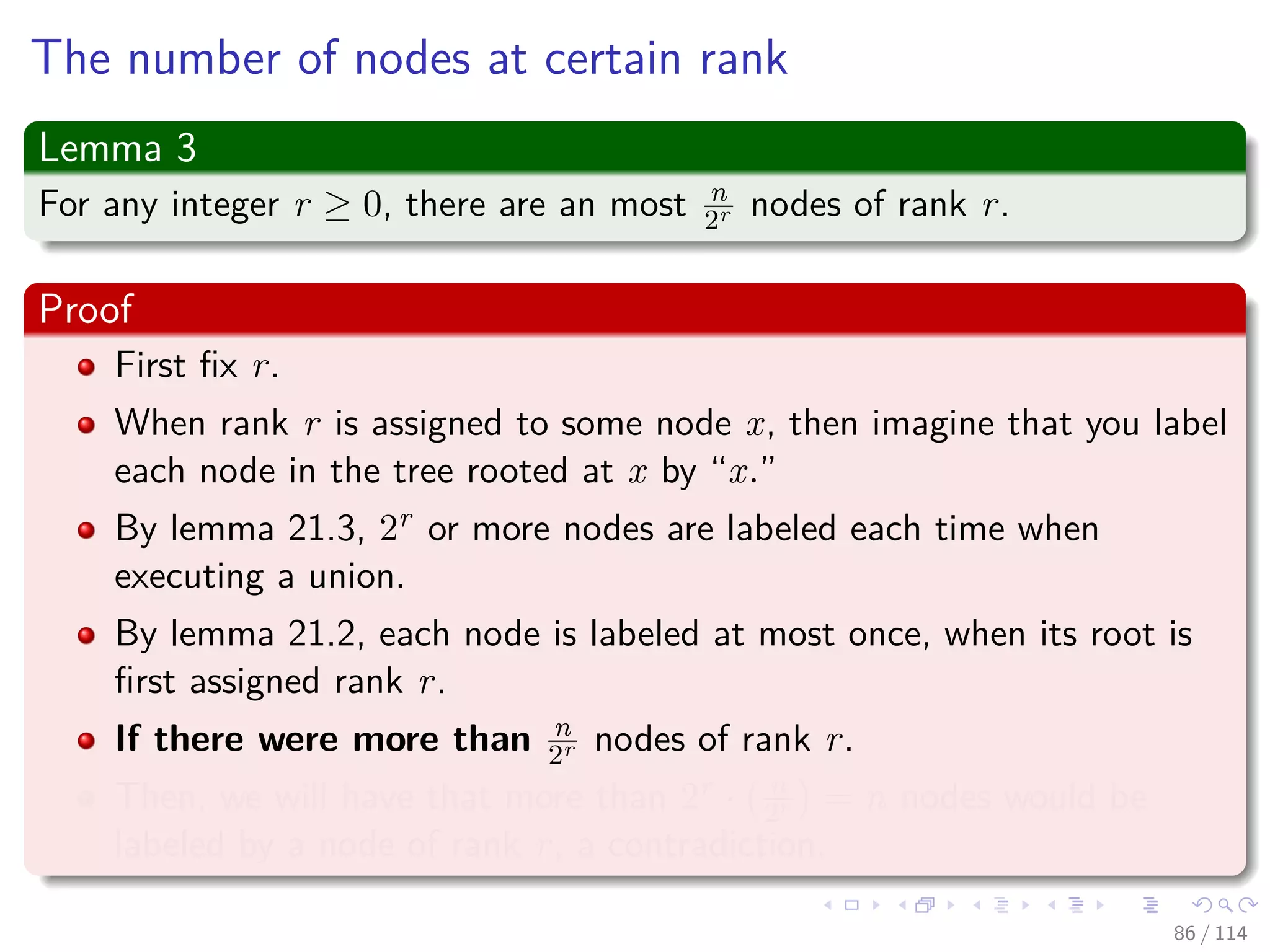
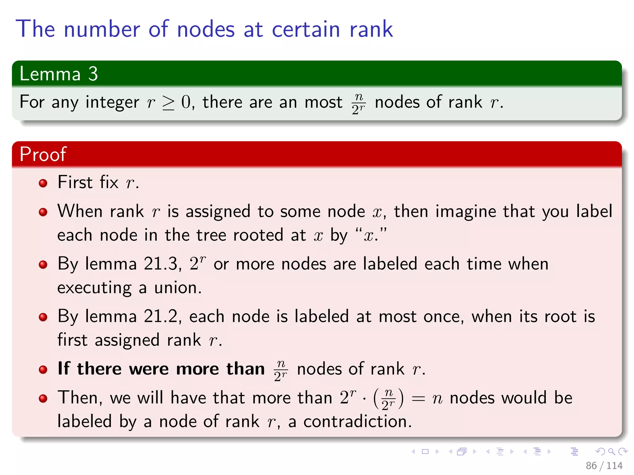
![The Number of Nodes in a Tree
Lemma 2
For all tree roots x, size(x) ≥ 2rank[x]
Note size (x)= Number of nodes in tree rooted at x
Proof
By induction on the number of link operations:
Basis Step
Before first link, all ranks are 0 and each tree contains one node.
Inductive Step
Consider linking x and y (Link (x, y))
Assume lemma holds before this operation; we show that it will holds
after.
81 / 114](https://image.slidesharecdn.com/17disjointsetrepresentation-151108151359-lva1-app6892/75/17-Disjoint-Set-Representation-197-2048.jpg)
![The Number of Nodes in a Tree
Lemma 2
For all tree roots x, size(x) ≥ 2rank[x]
Note size (x)= Number of nodes in tree rooted at x
Proof
By induction on the number of link operations:
Basis Step
Before first link, all ranks are 0 and each tree contains one node.
Inductive Step
Consider linking x and y (Link (x, y))
Assume lemma holds before this operation; we show that it will holds
after.
81 / 114](https://image.slidesharecdn.com/17disjointsetrepresentation-151108151359-lva1-app6892/75/17-Disjoint-Set-Representation-198-2048.jpg)
![The Number of Nodes in a Tree
Lemma 2
For all tree roots x, size(x) ≥ 2rank[x]
Note size (x)= Number of nodes in tree rooted at x
Proof
By induction on the number of link operations:
Basis Step
Before first link, all ranks are 0 and each tree contains one node.
Inductive Step
Consider linking x and y (Link (x, y))
Assume lemma holds before this operation; we show that it will holds
after.
81 / 114](https://image.slidesharecdn.com/17disjointsetrepresentation-151108151359-lva1-app6892/75/17-Disjoint-Set-Representation-199-2048.jpg)
![The Number of Nodes in a Tree
Lemma 2
For all tree roots x, size(x) ≥ 2rank[x]
Note size (x)= Number of nodes in tree rooted at x
Proof
By induction on the number of link operations:
Basis Step
Before first link, all ranks are 0 and each tree contains one node.
Inductive Step
Consider linking x and y (Link (x, y))
Assume lemma holds before this operation; we show that it will holds
after.
81 / 114](https://image.slidesharecdn.com/17disjointsetrepresentation-151108151359-lva1-app6892/75/17-Disjoint-Set-Representation-200-2048.jpg)
![The Number of Nodes in a Tree
Lemma 2
For all tree roots x, size(x) ≥ 2rank[x]
Note size (x)= Number of nodes in tree rooted at x
Proof
By induction on the number of link operations:
Basis Step
Before first link, all ranks are 0 and each tree contains one node.
Inductive Step
Consider linking x and y (Link (x, y))
Assume lemma holds before this operation; we show that it will holds
after.
81 / 114](https://image.slidesharecdn.com/17disjointsetrepresentation-151108151359-lva1-app6892/75/17-Disjoint-Set-Representation-201-2048.jpg)
![The Number of Nodes in a Tree
Lemma 2
For all tree roots x, size(x) ≥ 2rank[x]
Note size (x)= Number of nodes in tree rooted at x
Proof
By induction on the number of link operations:
Basis Step
Before first link, all ranks are 0 and each tree contains one node.
Inductive Step
Consider linking x and y (Link (x, y))
Assume lemma holds before this operation; we show that it will holds
after.
81 / 114](https://image.slidesharecdn.com/17disjointsetrepresentation-151108151359-lva1-app6892/75/17-Disjoint-Set-Representation-202-2048.jpg)
![The Number of Nodes in a Tree
Lemma 2
For all tree roots x, size(x) ≥ 2rank[x]
Note size (x)= Number of nodes in tree rooted at x
Proof
By induction on the number of link operations:
Basis Step
Before first link, all ranks are 0 and each tree contains one node.
Inductive Step
Consider linking x and y (Link (x, y))
Assume lemma holds before this operation; we show that it will holds
after.
81 / 114](https://image.slidesharecdn.com/17disjointsetrepresentation-151108151359-lva1-app6892/75/17-Disjoint-Set-Representation-203-2048.jpg)
![Case 1: rank[x] = rank[y]
Assume rank [x] < rank [y]
Note:
rank [x] == rank [x] and rank [y] == rank [y]
82 / 114](https://image.slidesharecdn.com/17disjointsetrepresentation-151108151359-lva1-app6892/75/17-Disjoint-Set-Representation-204-2048.jpg)
![Therefore
We have that
size (y) = size (x) + size (y)
≥ 2rank[x]
+ 2rank[y]
≥ 2rank[y]
= 2rank [y]
83 / 114](https://image.slidesharecdn.com/17disjointsetrepresentation-151108151359-lva1-app6892/75/17-Disjoint-Set-Representation-205-2048.jpg)
![Therefore
We have that
size (y) = size (x) + size (y)
≥ 2rank[x]
+ 2rank[y]
≥ 2rank[y]
= 2rank [y]
83 / 114](https://image.slidesharecdn.com/17disjointsetrepresentation-151108151359-lva1-app6892/75/17-Disjoint-Set-Representation-206-2048.jpg)
![Therefore
We have that
size (y) = size (x) + size (y)
≥ 2rank[x]
+ 2rank[y]
≥ 2rank[y]
= 2rank [y]
83 / 114](https://image.slidesharecdn.com/17disjointsetrepresentation-151108151359-lva1-app6892/75/17-Disjoint-Set-Representation-207-2048.jpg)
![Therefore
We have that
size (y) = size (x) + size (y)
≥ 2rank[x]
+ 2rank[y]
≥ 2rank[y]
= 2rank [y]
83 / 114](https://image.slidesharecdn.com/17disjointsetrepresentation-151108151359-lva1-app6892/75/17-Disjoint-Set-Representation-208-2048.jpg)
![Case 2: rank[x] == rank[y]
Assume rank [x] == rank [y]
Note:
rank [x] == rank [x] and rank [y] == rank [y] + 1
84 / 114](https://image.slidesharecdn.com/17disjointsetrepresentation-151108151359-lva1-app6892/75/17-Disjoint-Set-Representation-209-2048.jpg)
![Therefore
We have that
size (y) = size (x) + size (y)
≥ 2rank[x]
+ 2rank[y]
≥ 2rank[y]+1
= 2rank [y]
Note: In the worst case rank [x] == rank [y] == 0
85 / 114](https://image.slidesharecdn.com/17disjointsetrepresentation-151108151359-lva1-app6892/75/17-Disjoint-Set-Representation-210-2048.jpg)
![Therefore
We have that
size (y) = size (x) + size (y)
≥ 2rank[x]
+ 2rank[y]
≥ 2rank[y]+1
= 2rank [y]
Note: In the worst case rank [x] == rank [y] == 0
85 / 114](https://image.slidesharecdn.com/17disjointsetrepresentation-151108151359-lva1-app6892/75/17-Disjoint-Set-Representation-211-2048.jpg)
![Therefore
We have that
size (y) = size (x) + size (y)
≥ 2rank[x]
+ 2rank[y]
≥ 2rank[y]+1
= 2rank [y]
Note: In the worst case rank [x] == rank [y] == 0
85 / 114](https://image.slidesharecdn.com/17disjointsetrepresentation-151108151359-lva1-app6892/75/17-Disjoint-Set-Representation-212-2048.jpg)
![Therefore
We have that
size (y) = size (x) + size (y)
≥ 2rank[x]
+ 2rank[y]
≥ 2rank[y]+1
= 2rank [y]
Note: In the worst case rank [x] == rank [y] == 0
85 / 114](https://image.slidesharecdn.com/17disjointsetrepresentation-151108151359-lva1-app6892/75/17-Disjoint-Set-Representation-213-2048.jpg)
![Therefore
We have that
size (y) = size (x) + size (y)
≥ 2rank[x]
+ 2rank[y]
≥ 2rank[y]+1
= 2rank [y]
Note: In the worst case rank [x] == rank [y] == 0
85 / 114](https://image.slidesharecdn.com/17disjointsetrepresentation-151108151359-lva1-app6892/75/17-Disjoint-Set-Representation-214-2048.jpg)


![Proof
Proof
Given a node x, we know that:
rank [p [x]] − rank [x] is monotonically increasing ⇒
log∗
rank [p [x]] − log∗
rank [x] is monotonically increasing.
Thus, Once x and p[x] are in different blocks, they will always be in
different blocks because:
The rank of the parent can only increases.
And the child’s rank stays the same
Thus, the node x will be billed in the first FindSet operation a patch
charge and block charge if necessary.
Thus, the node x will never be charged again a path charge because
is already pointing to the member set name.
105 / 114](https://image.slidesharecdn.com/17disjointsetrepresentation-151108151359-lva1-app6892/75/17-Disjoint-Set-Representation-267-2048.jpg)
![Proof
Proof
Given a node x, we know that:
rank [p [x]] − rank [x] is monotonically increasing ⇒
log∗
rank [p [x]] − log∗
rank [x] is monotonically increasing.
Thus, Once x and p[x] are in different blocks, they will always be in
different blocks because:
The rank of the parent can only increases.
And the child’s rank stays the same
Thus, the node x will be billed in the first FindSet operation a patch
charge and block charge if necessary.
Thus, the node x will never be charged again a path charge because
is already pointing to the member set name.
105 / 114](https://image.slidesharecdn.com/17disjointsetrepresentation-151108151359-lva1-app6892/75/17-Disjoint-Set-Representation-268-2048.jpg)
![Proof
Proof
Given a node x, we know that:
rank [p [x]] − rank [x] is monotonically increasing ⇒
log∗
rank [p [x]] − log∗
rank [x] is monotonically increasing.
Thus, Once x and p[x] are in different blocks, they will always be in
different blocks because:
The rank of the parent can only increases.
And the child’s rank stays the same
Thus, the node x will be billed in the first FindSet operation a patch
charge and block charge if necessary.
Thus, the node x will never be charged again a path charge because
is already pointing to the member set name.
105 / 114](https://image.slidesharecdn.com/17disjointsetrepresentation-151108151359-lva1-app6892/75/17-Disjoint-Set-Representation-269-2048.jpg)
![Proof
Proof
Given a node x, we know that:
rank [p [x]] − rank [x] is monotonically increasing ⇒
log∗
rank [p [x]] − log∗
rank [x] is monotonically increasing.
Thus, Once x and p[x] are in different blocks, they will always be in
different blocks because:
The rank of the parent can only increases.
And the child’s rank stays the same
Thus, the node x will be billed in the first FindSet operation a patch
charge and block charge if necessary.
Thus, the node x will never be charged again a path charge because
is already pointing to the member set name.
105 / 114](https://image.slidesharecdn.com/17disjointsetrepresentation-151108151359-lva1-app6892/75/17-Disjoint-Set-Representation-270-2048.jpg)
![Proof
Proof
Given a node x, we know that:
rank [p [x]] − rank [x] is monotonically increasing ⇒
log∗
rank [p [x]] − log∗
rank [x] is monotonically increasing.
Thus, Once x and p[x] are in different blocks, they will always be in
different blocks because:
The rank of the parent can only increases.
And the child’s rank stays the same
Thus, the node x will be billed in the first FindSet operation a patch
charge and block charge if necessary.
Thus, the node x will never be charged again a path charge because
is already pointing to the member set name.
105 / 114](https://image.slidesharecdn.com/17disjointsetrepresentation-151108151359-lva1-app6892/75/17-Disjoint-Set-Representation-271-2048.jpg)
![Proof
Proof
Given a node x, we know that:
rank [p [x]] − rank [x] is monotonically increasing ⇒
log∗
rank [p [x]] − log∗
rank [x] is monotonically increasing.
Thus, Once x and p[x] are in different blocks, they will always be in
different blocks because:
The rank of the parent can only increases.
And the child’s rank stays the same
Thus, the node x will be billed in the first FindSet operation a patch
charge and block charge if necessary.
Thus, the node x will never be charged again a path charge because
is already pointing to the member set name.
105 / 114](https://image.slidesharecdn.com/17disjointsetrepresentation-151108151359-lva1-app6892/75/17-Disjoint-Set-Representation-272-2048.jpg)
![Proof
Proof
Given a node x, we know that:
rank [p [x]] − rank [x] is monotonically increasing ⇒
log∗
rank [p [x]] − log∗
rank [x] is monotonically increasing.
Thus, Once x and p[x] are in different blocks, they will always be in
different blocks because:
The rank of the parent can only increases.
And the child’s rank stays the same
Thus, the node x will be billed in the first FindSet operation a patch
charge and block charge if necessary.
Thus, the node x will never be charged again a path charge because
is already pointing to the member set name.
105 / 114](https://image.slidesharecdn.com/17disjointsetrepresentation-151108151359-lva1-app6892/75/17-Disjoint-Set-Representation-273-2048.jpg)


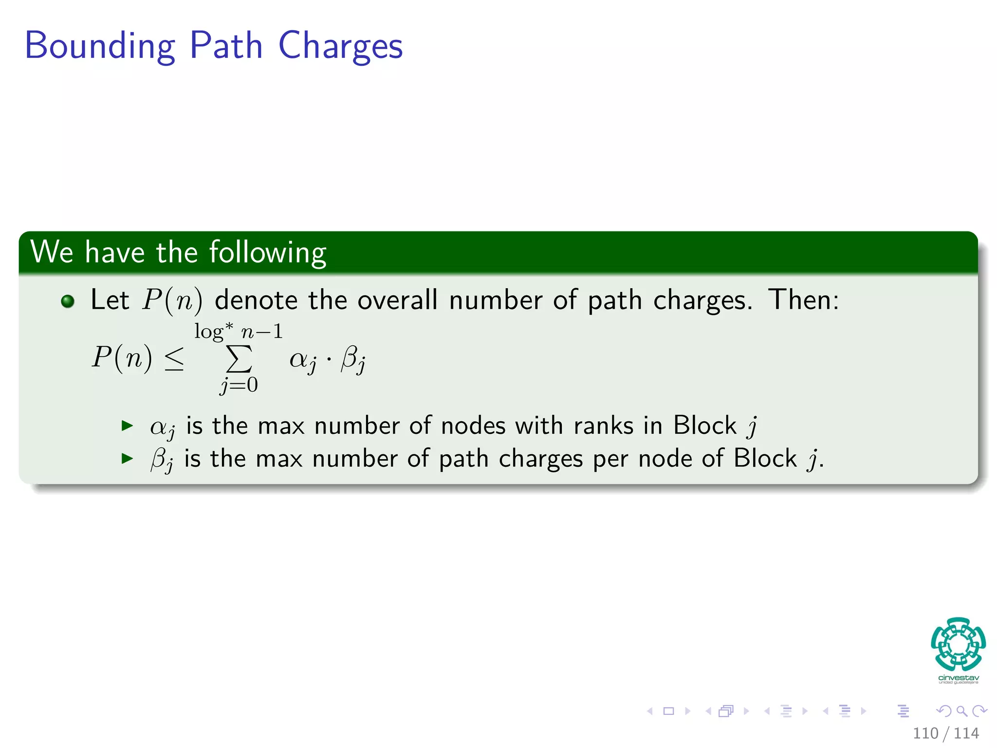
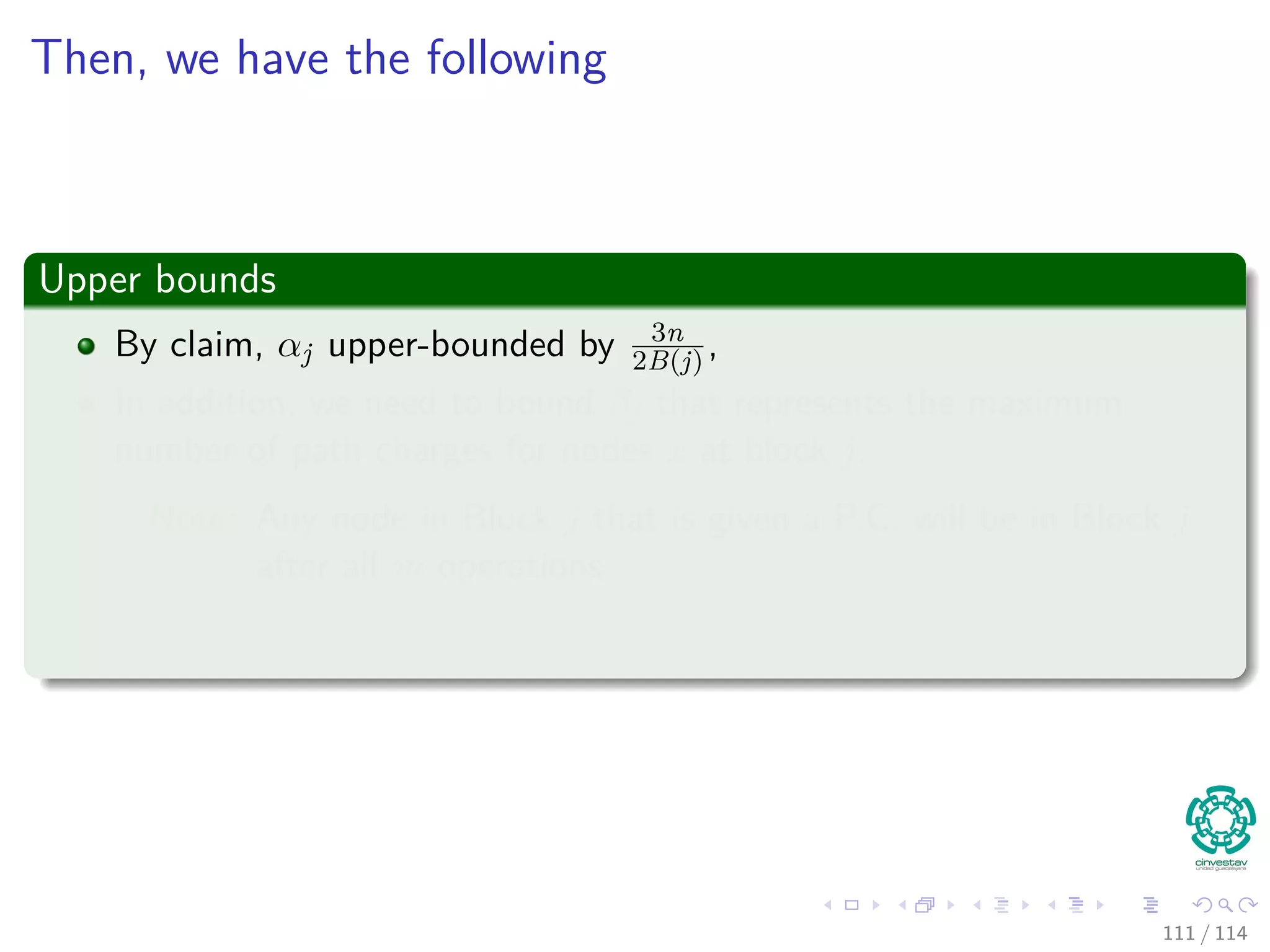
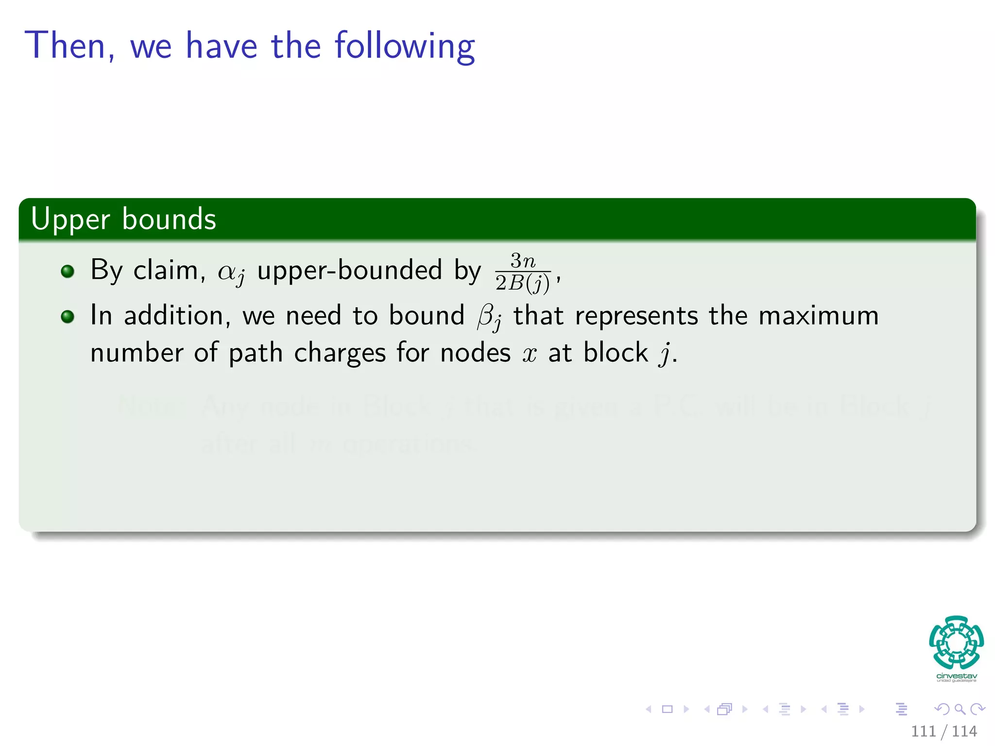
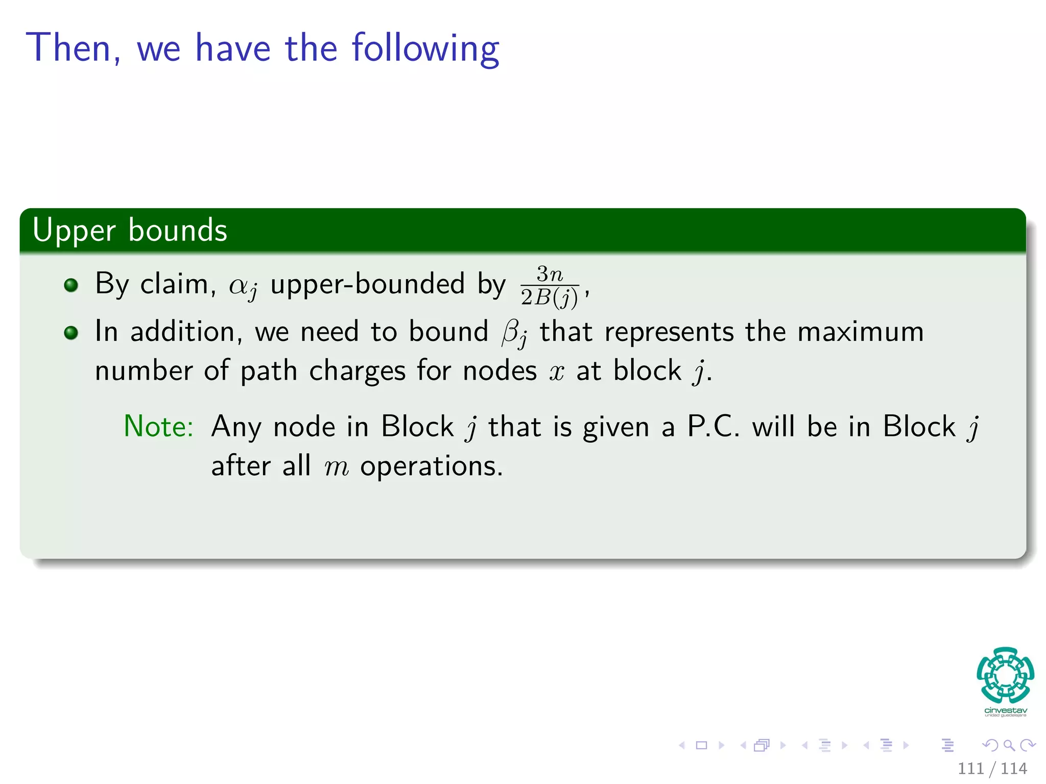


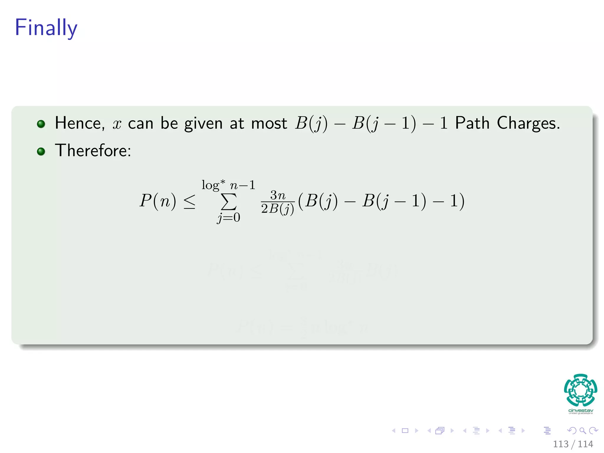
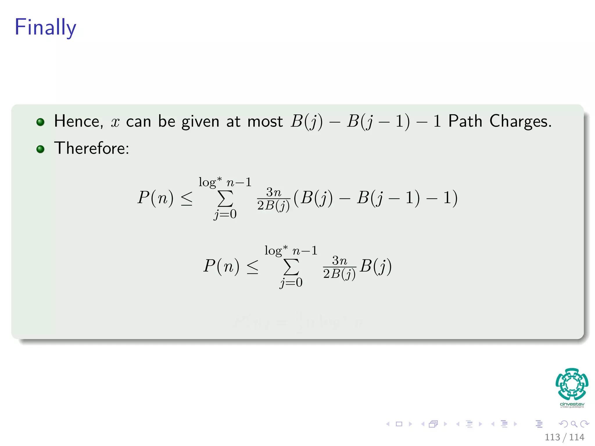
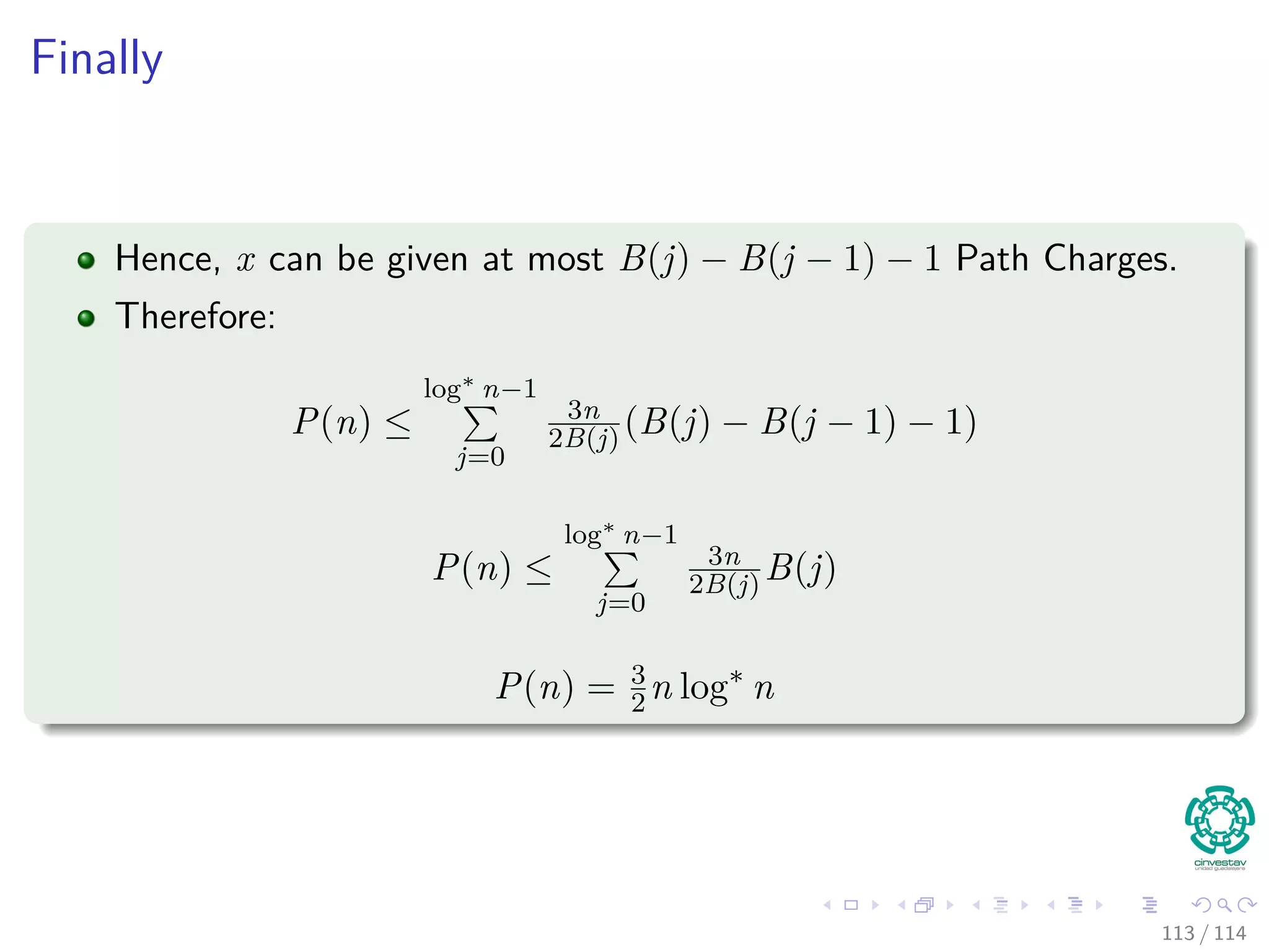
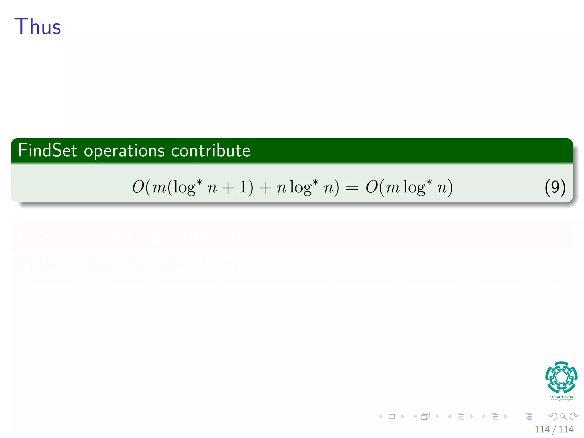

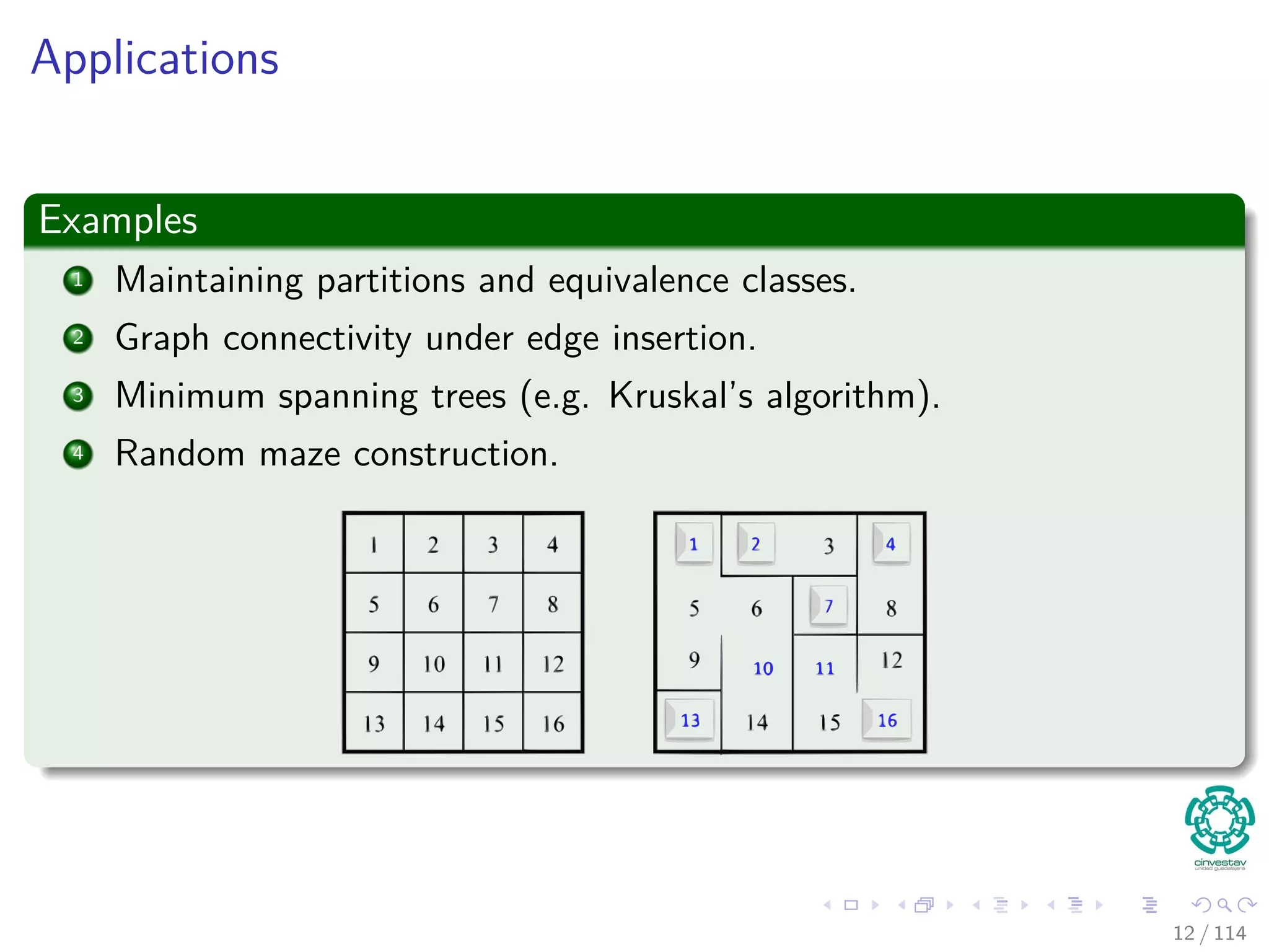
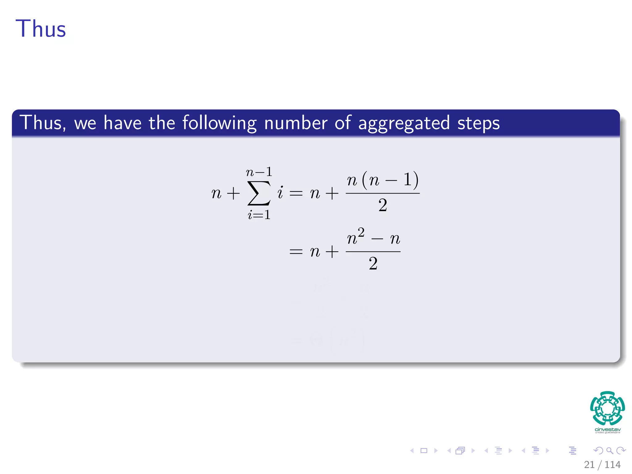
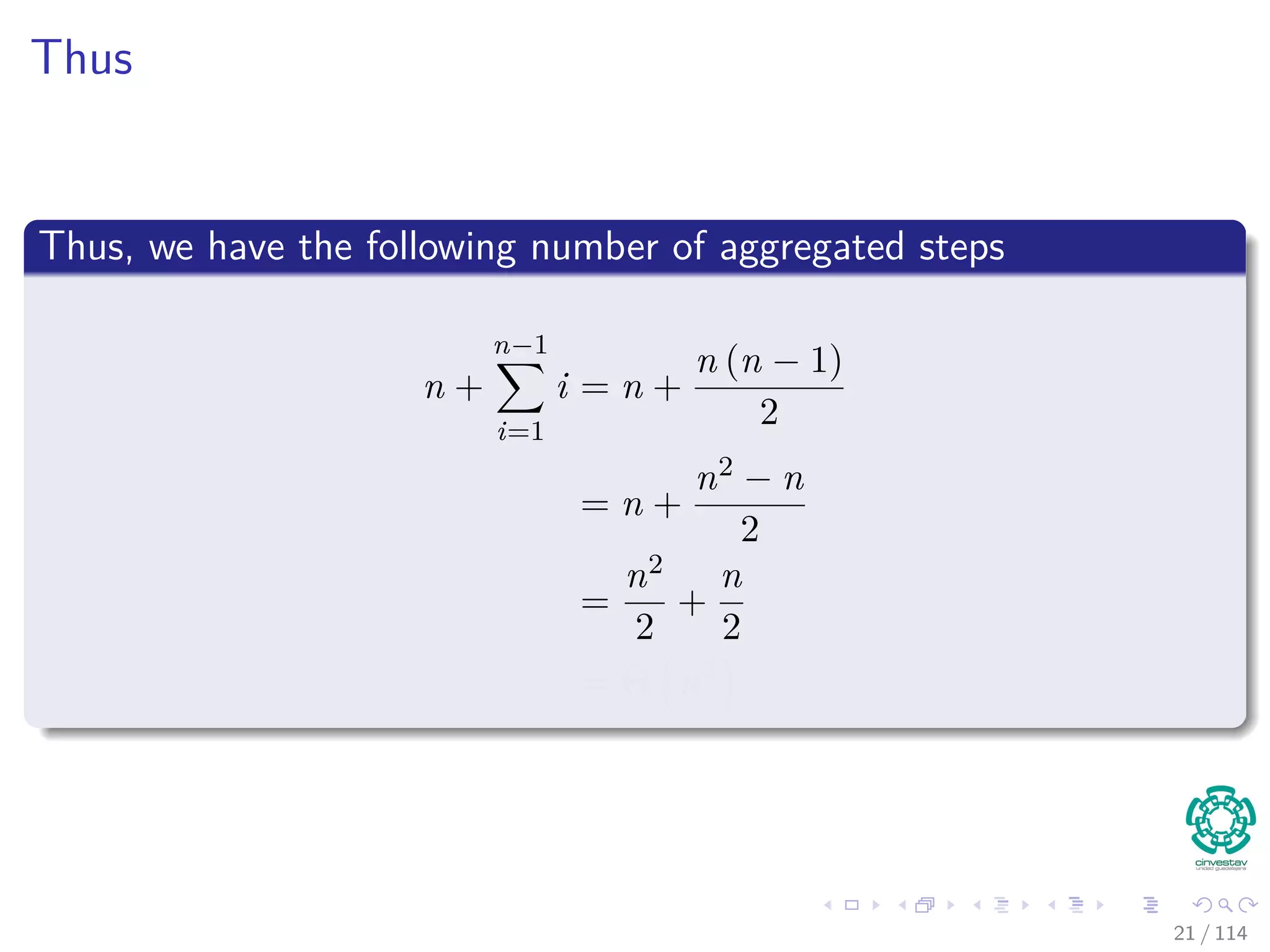
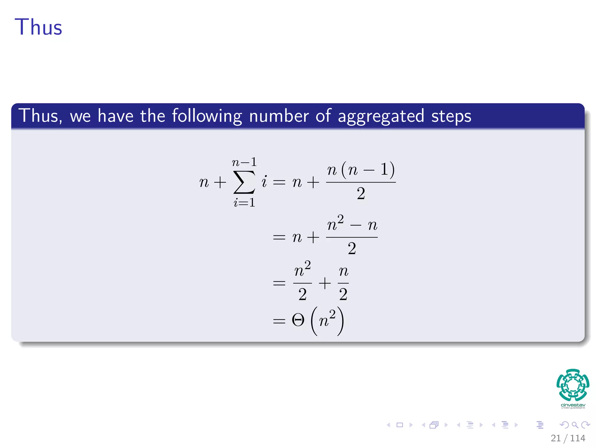
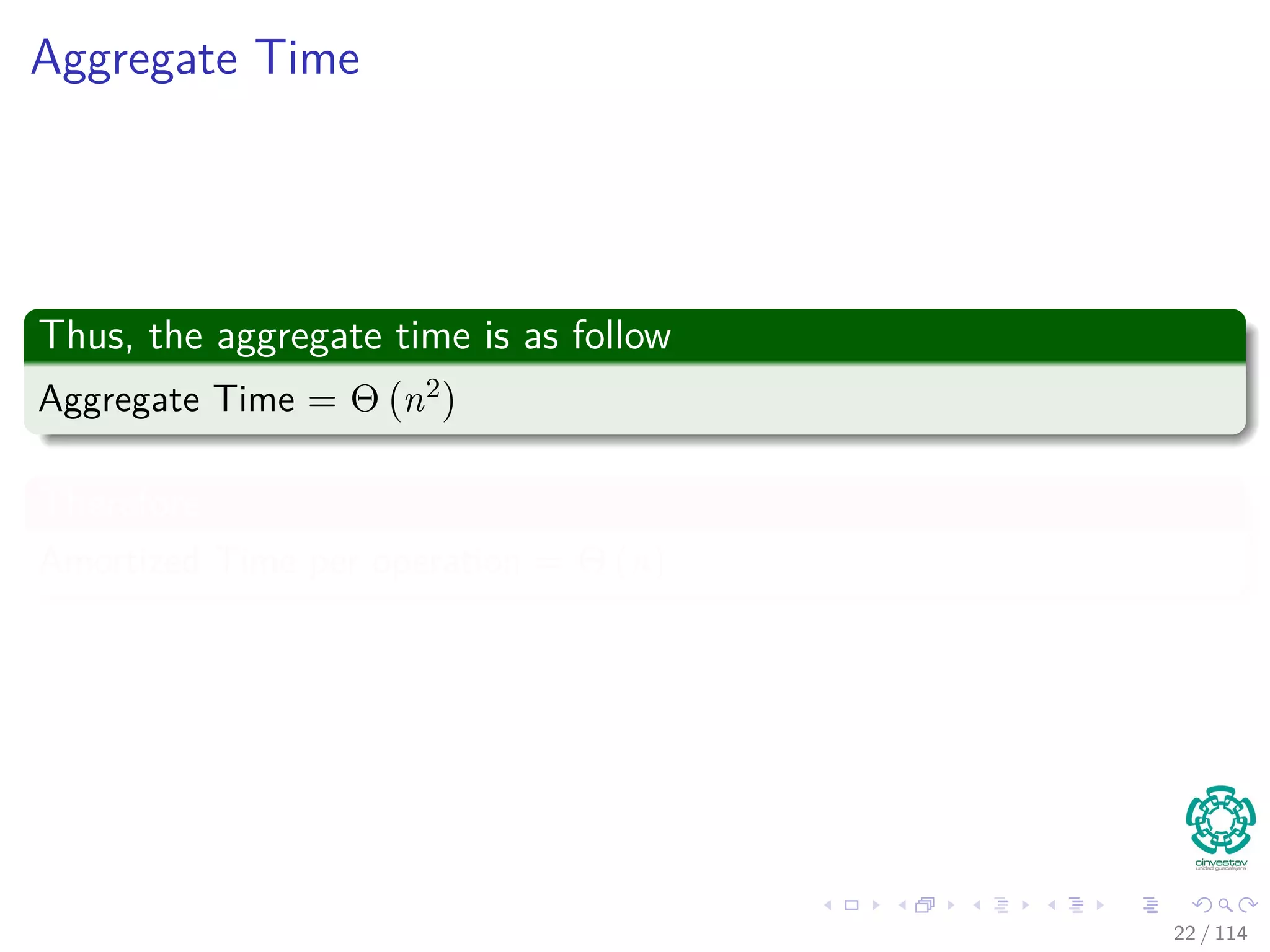
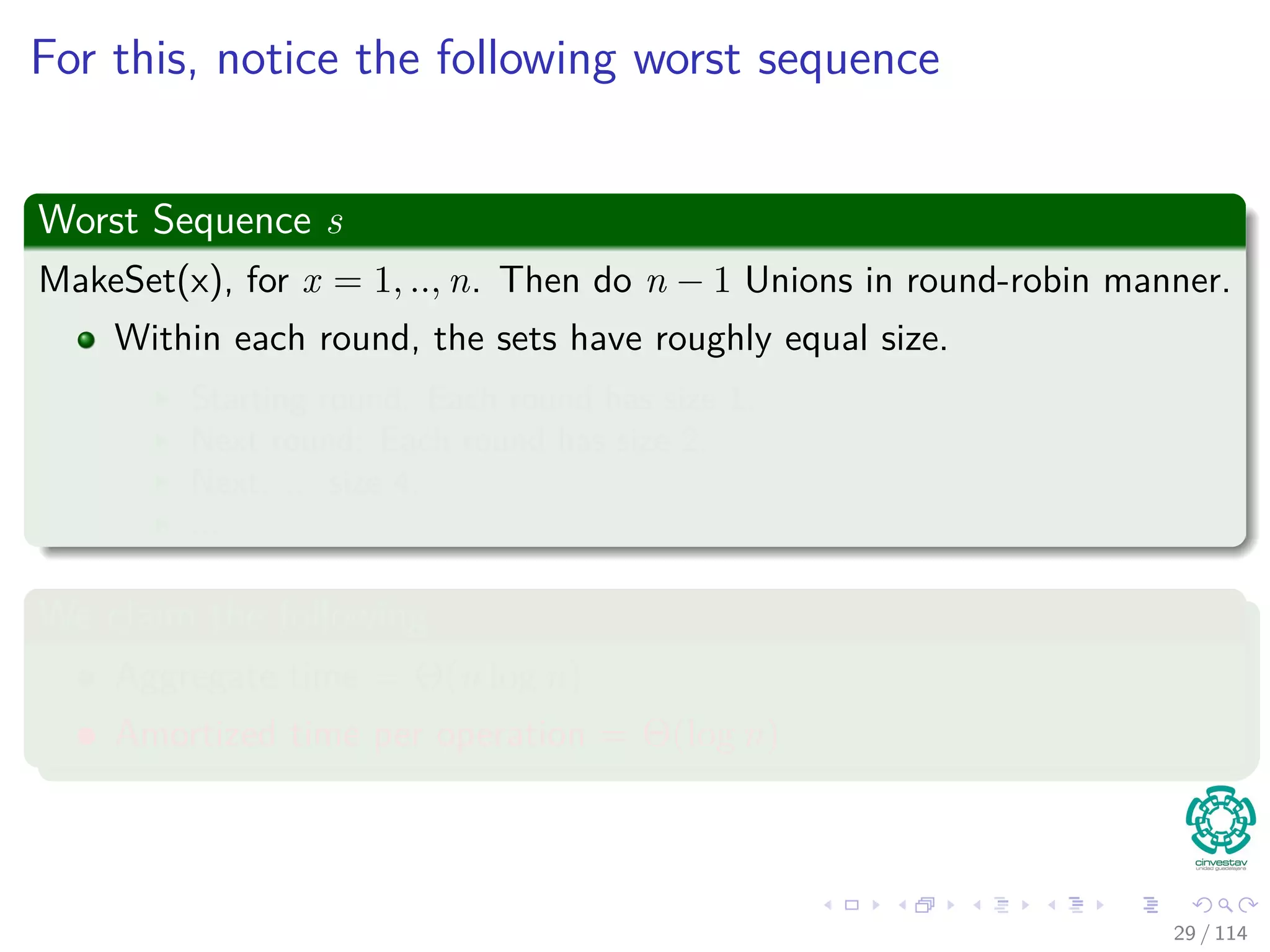
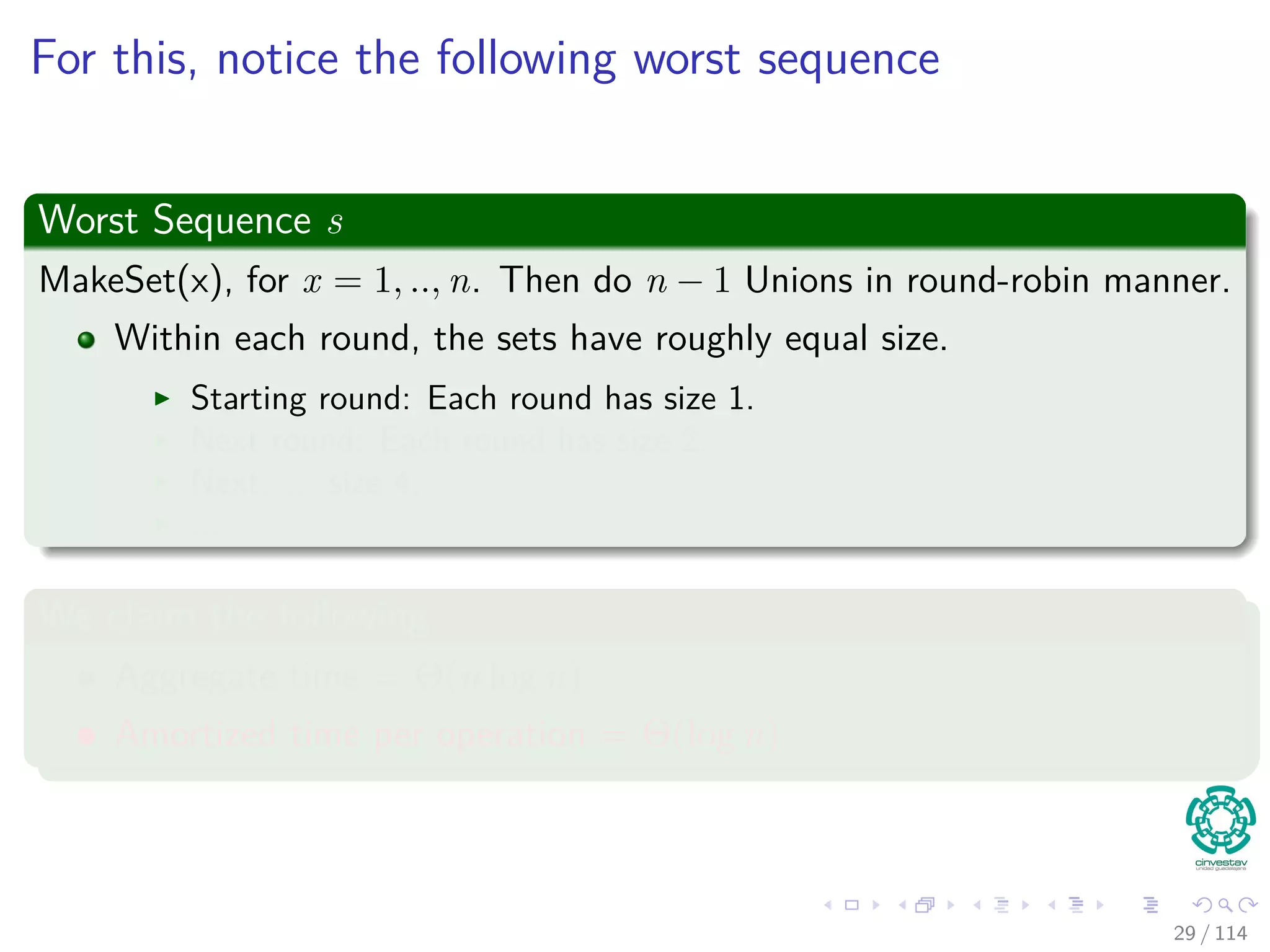
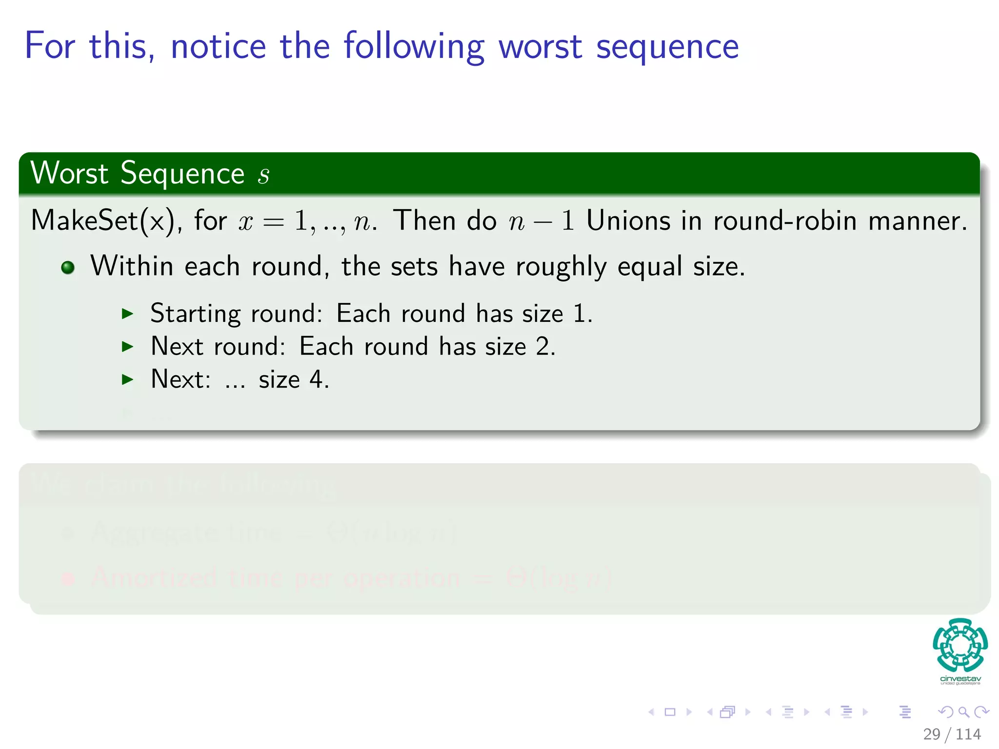
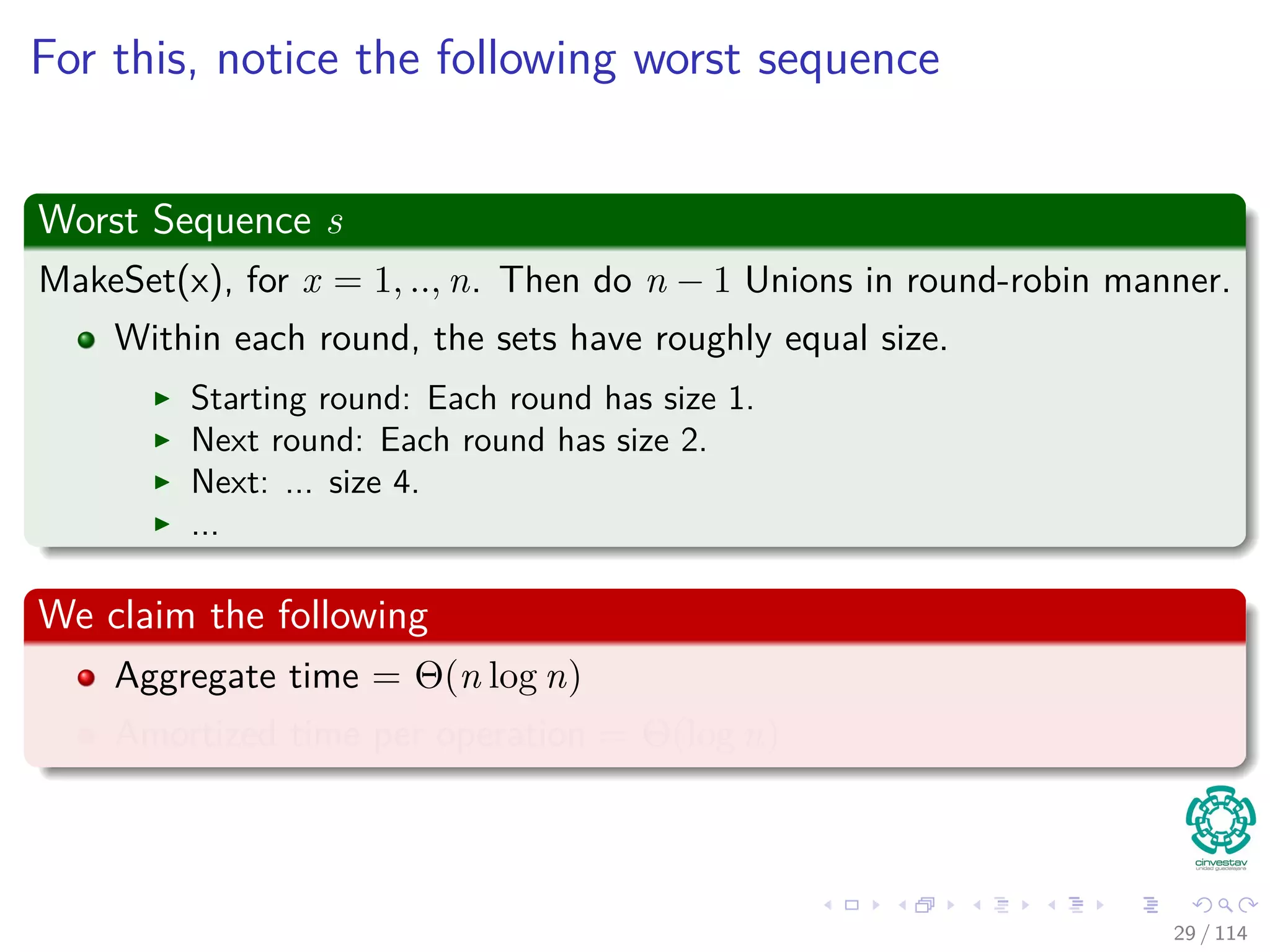
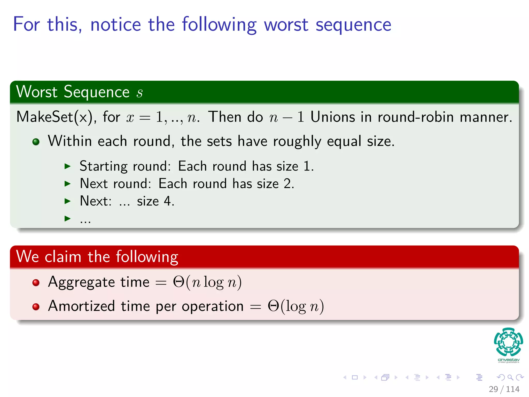
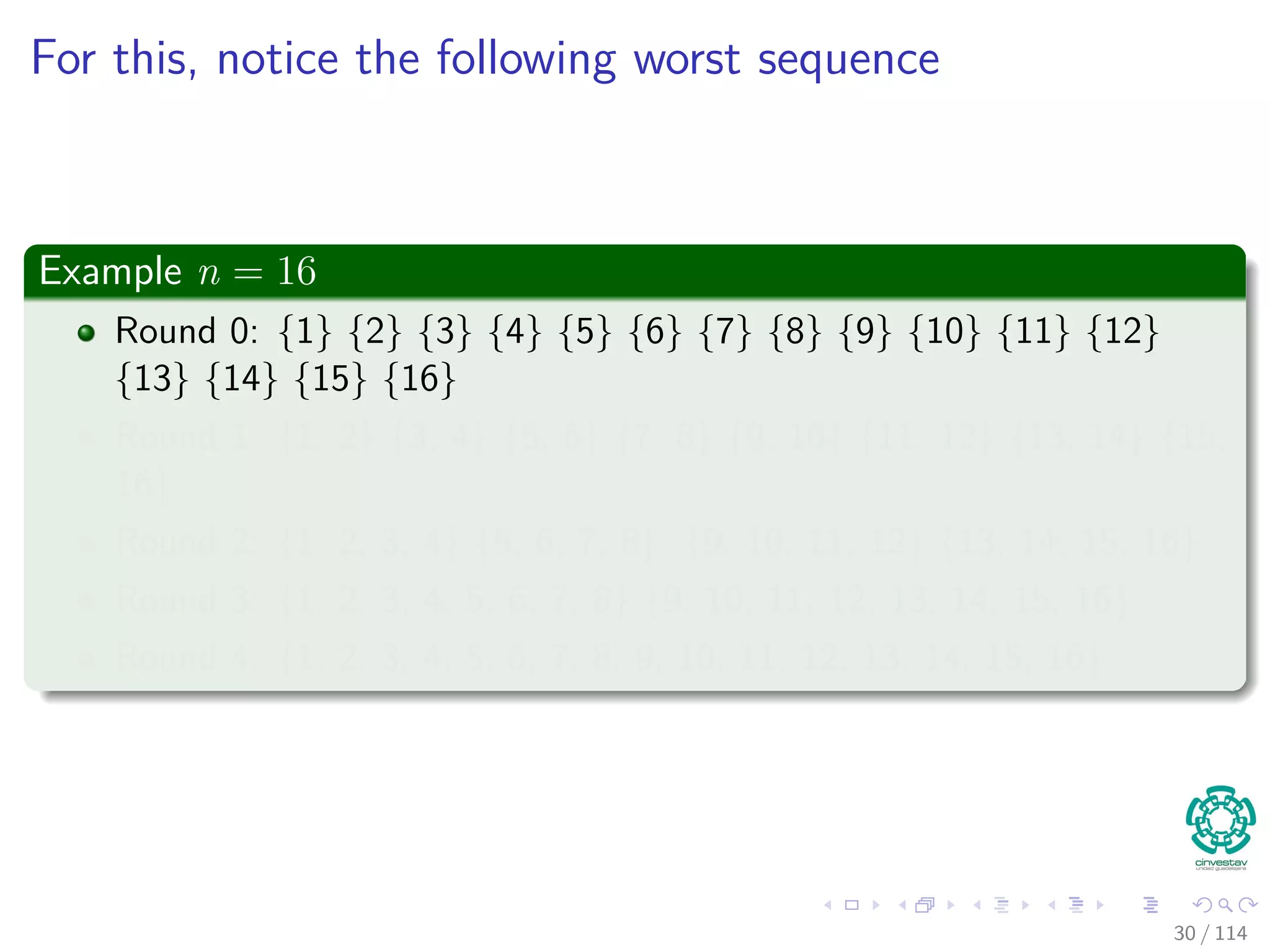
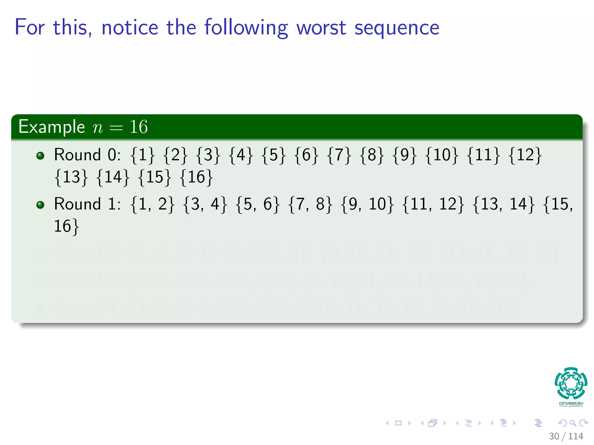
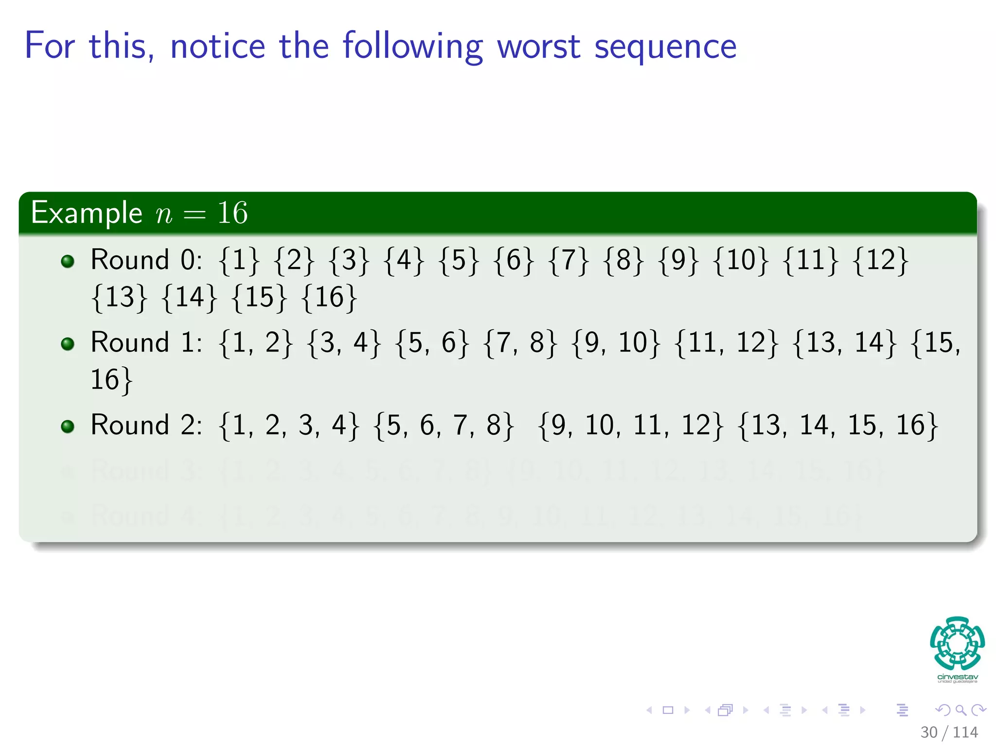
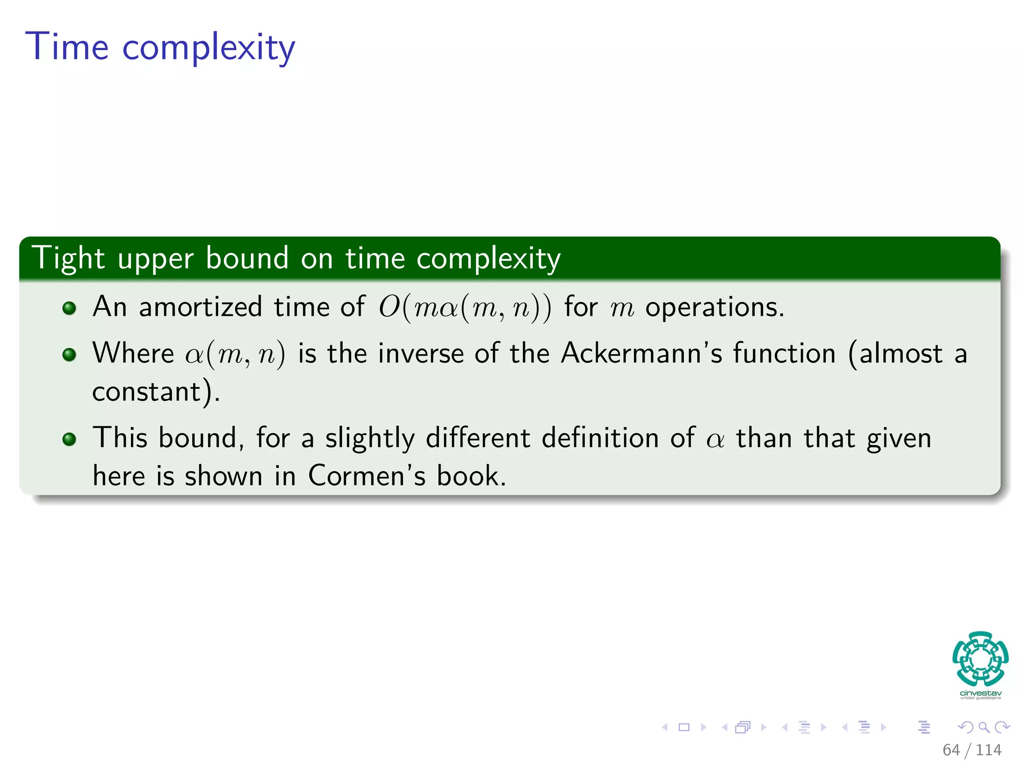
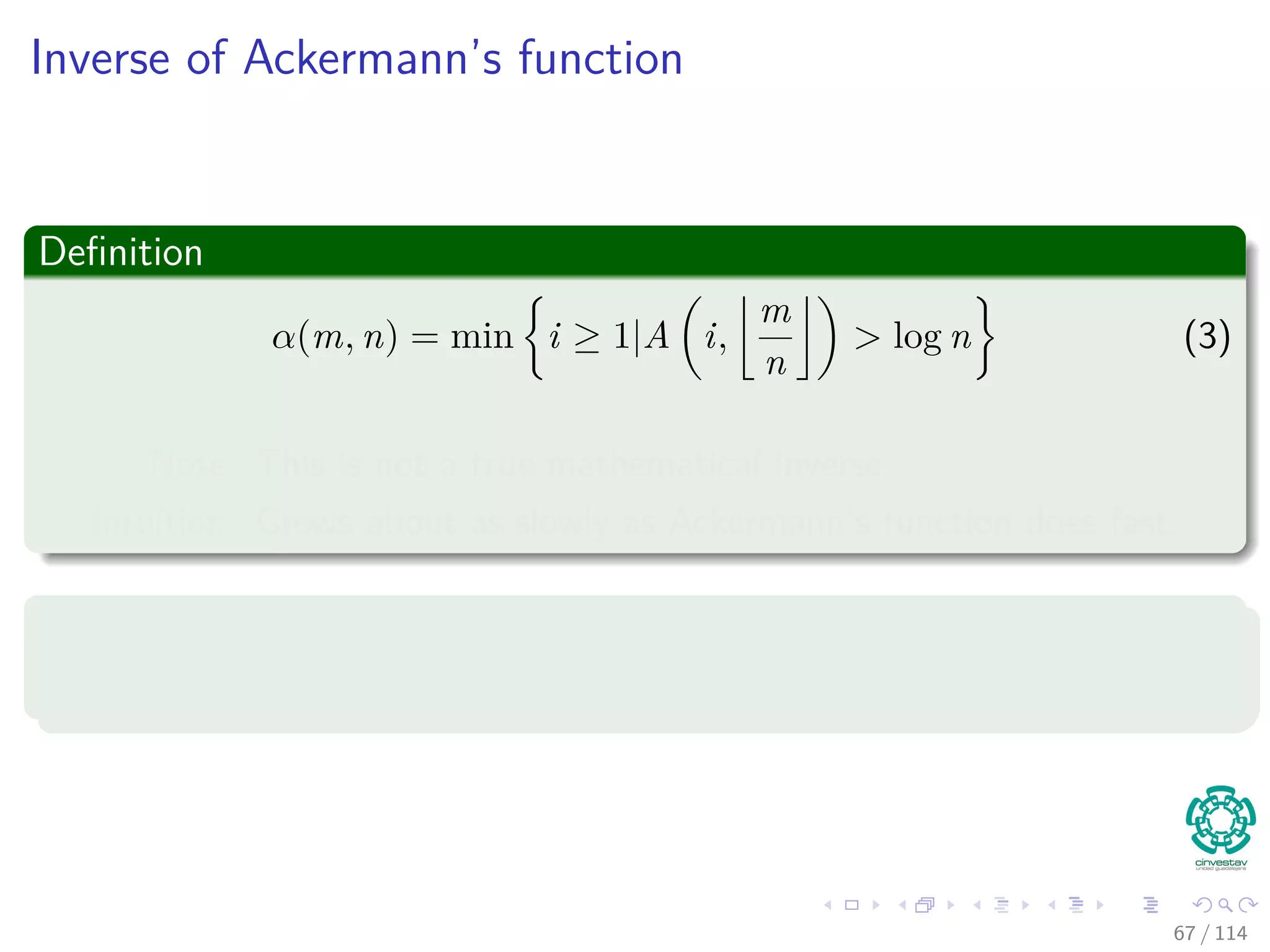
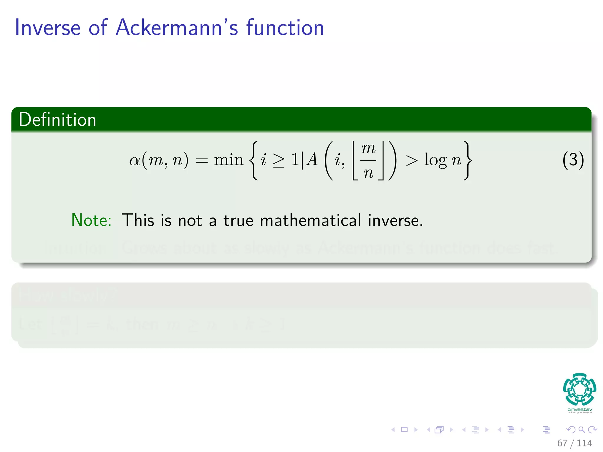
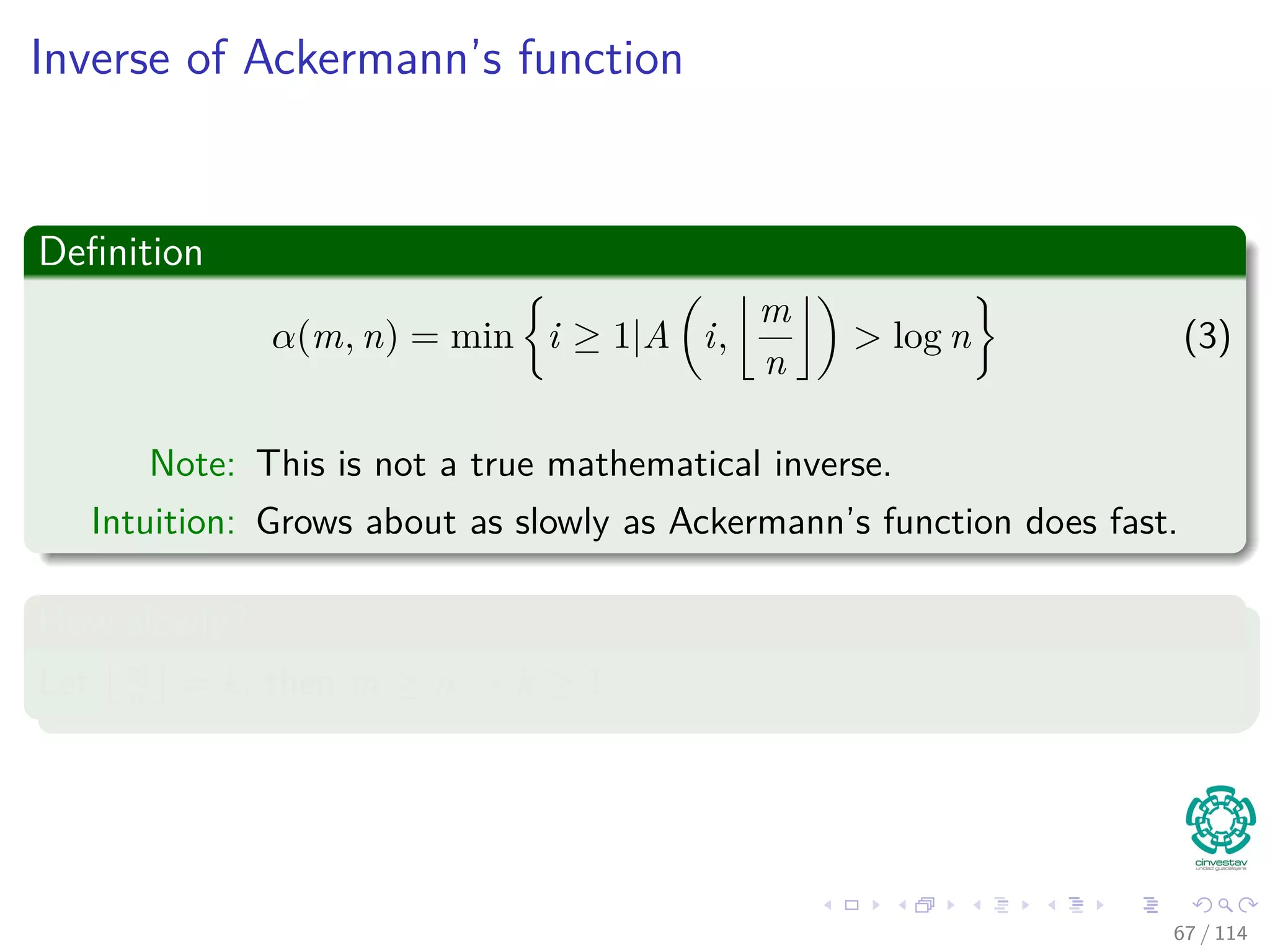
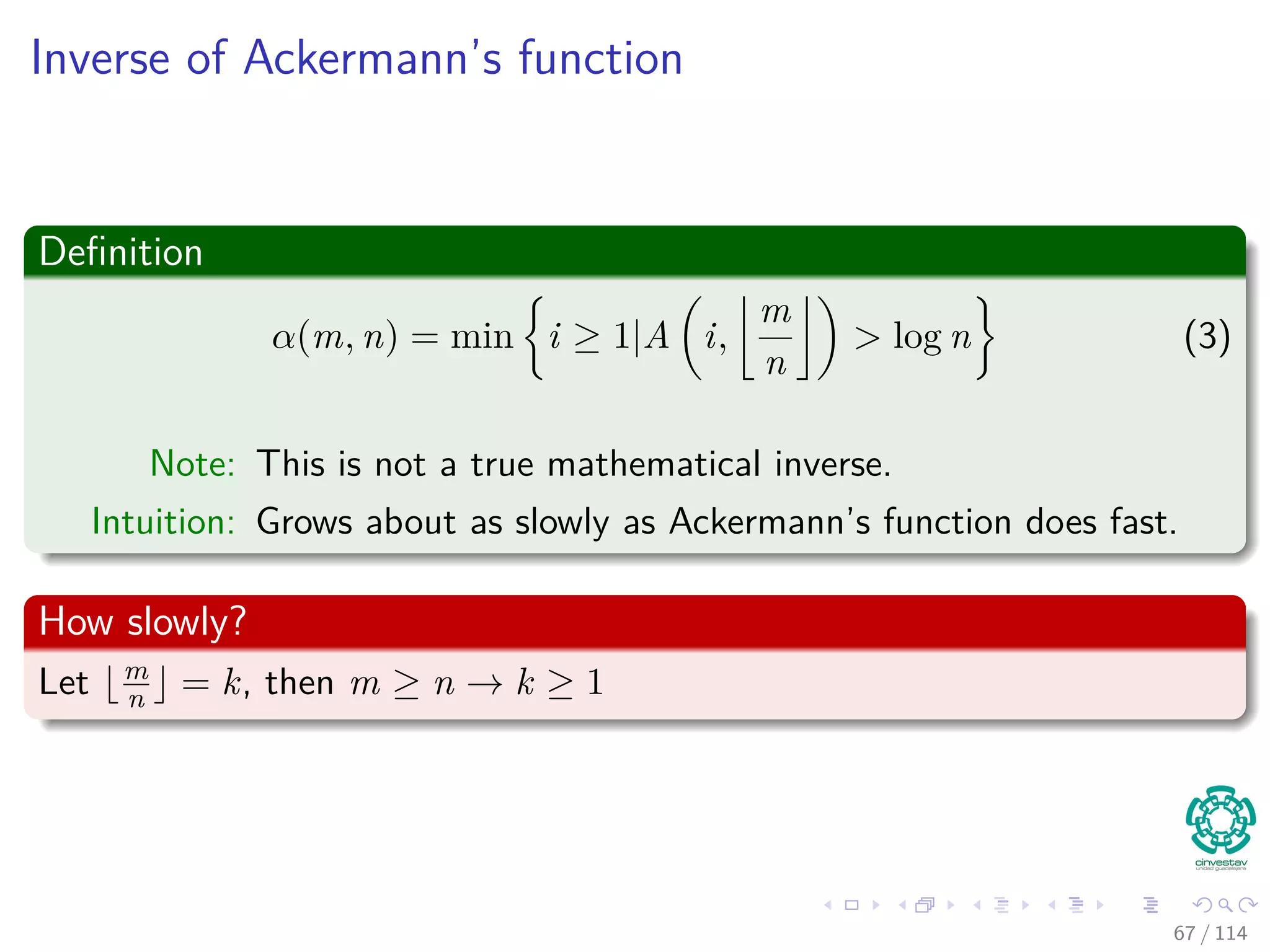
The document discusses the disjoint set representation and its applications, primarily focusing on the union-find problem and its operations: makeset, union, and find. It covers various implementations and optimizations such as weighted-union and path compression to improve the time complexity of these operations. Additionally, the document explores its applications in maintaining equivalence classes, graph connectivity, and minimum spanning trees.