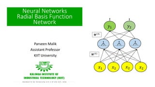
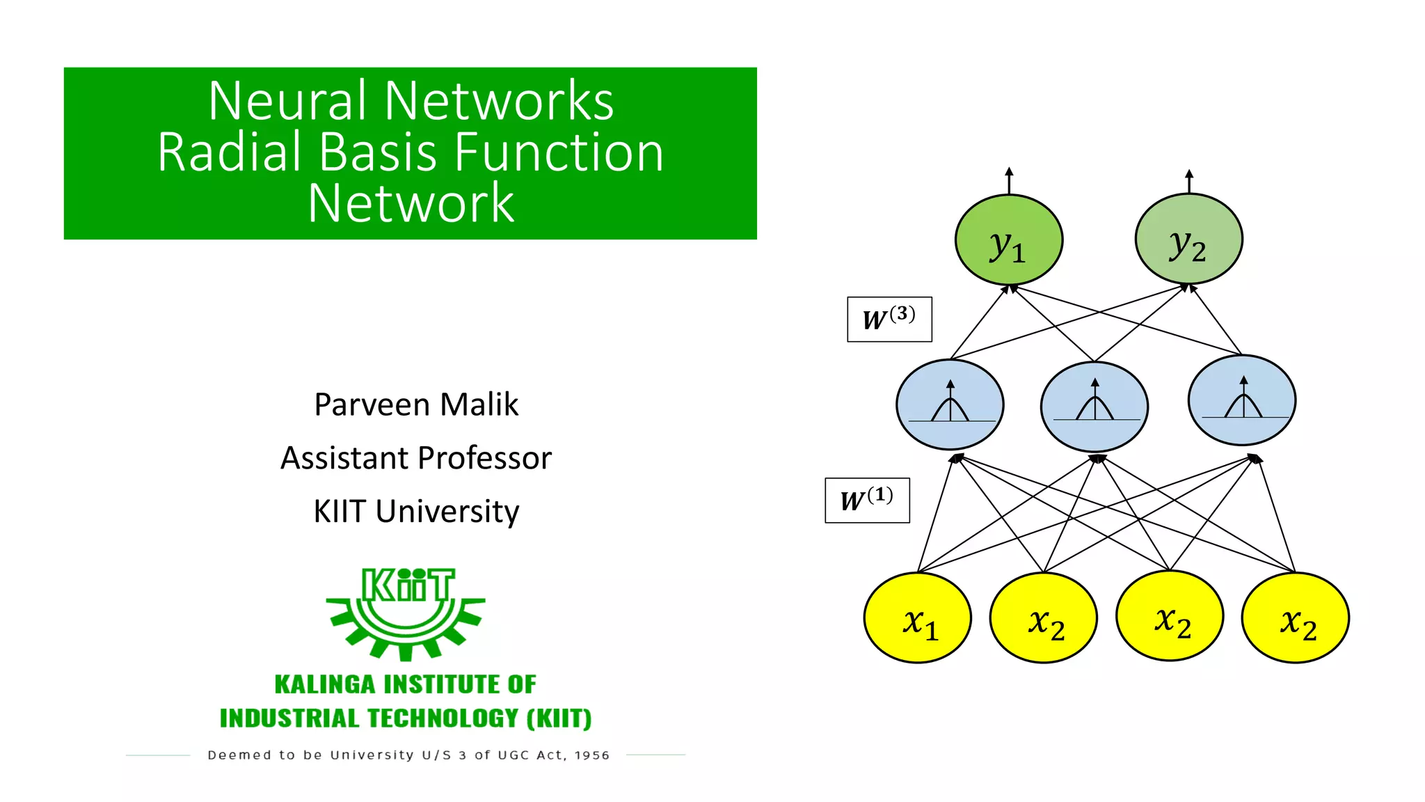
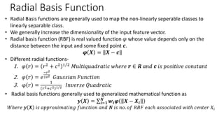
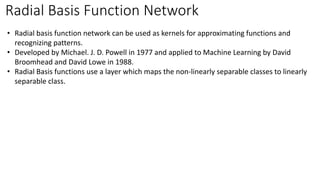
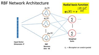
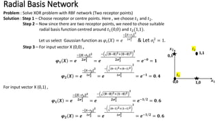
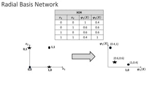
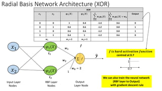
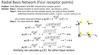
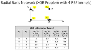
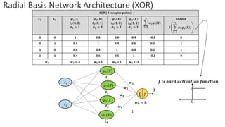
Parveen Malik
Assistant Professor
KIIT University
Neural Networks
Radial Basis Function
Network
𝑥1 𝑥2 𝑥2 𝑥2
𝑦1 𝑦2
𝑾(𝟏)
𝑾(𝟑)
Radial Basis Function
• Radial Basis functions are generally used to map the non-linearly seperable classes to
linearly separable class.
• We generally increase the dimensionality of the input feature vector.
• Radial basis function (RBF) is real valued function 𝜑 whose value depends only on the
distance between the input and some fixed point 𝒄.
𝝋 𝑿 = 𝑿 − 𝒄
• Different radial functions-
1. 𝜑 𝑟 = 𝑟2 + 𝑐2 Τ
1 2 𝑀𝑢𝑙𝑡𝑖𝑞𝑢𝑎𝑑𝑟𝑎𝑡𝑖𝑐 𝑤ℎ𝑒𝑟𝑒 𝒓 ∈ 𝑹 𝑎𝑛𝑑 𝒄 𝑖𝑠 𝑝𝑜𝑠𝑖𝑡𝑖𝑣𝑒 𝑐𝑜𝑛𝑠𝑡𝑎𝑛𝑡
2. 𝜑 𝑟 = 𝑒
−𝑟2
2𝜎2 𝐺𝑎𝑢𝑠𝑠𝑖𝑎𝑛 𝐹𝑢𝑛𝑐𝑡𝑖𝑜𝑛
3. φ 𝑟 =
1
𝑟2+𝑐2 Τ
1 2 𝐼𝑛𝑣𝑒𝑟𝑠𝑒 𝑄𝑢𝑎𝑑𝑟𝑎𝑡𝑖𝑐
• Radial basis functions generally used to generalized mathematical function as
𝒚 𝑿 = σ𝒊=𝟏
𝑵
𝒘𝒊𝝋 𝑿 − 𝑿𝒊
𝑊ℎ𝑒𝑟𝑒 𝒚 𝑿 𝑖𝑠 𝑎𝑝𝑝𝑟𝑜𝑥𝑖𝑚𝑎𝑡𝑖𝑛𝑔 𝑓𝑢𝑛𝑐𝑡𝑖𝑜𝑛 𝑎𝑛𝑑 𝑵 𝑖𝑠 𝑛𝑜. 𝑜𝑓 𝑅𝐵𝐹 𝑒𝑎𝑐ℎ 𝑎𝑠𝑠𝑜𝑐𝑖𝑎𝑡𝑒𝑑 𝑤𝑖𝑡ℎ 𝑐𝑒𝑛𝑡𝑒𝑟 𝑋𝑖
Radial Basis Function Network
• Radial basis function network can be used as kernels for approximating functions and
recognizing patterns.
• Developed by Michael. J. D. Powell in 1977 and applied to Machine Learning by David
Broomhead and David Lowe in 1988.
• Radial Basis functions use a layer which maps the non-linearly separable classes to linearly
separable class.
𝒕𝟏
𝒕𝟐
𝒕𝑴
∑
⋮
∑
Input Vector
Dimension -P RBF
Neurons
Dim - M
Weighted
Sums
RBF Network Architecture
⋮
𝒕𝒊 → 𝑹𝒆𝒄𝒆𝒑𝒕𝒐𝒓 𝒐𝒓 𝒄𝒆𝒏𝒕𝒓𝒆 𝒑𝒐𝒊𝒏𝒕
Radial basis function
𝝋𝒊 𝑿 = 𝒆
− 𝑿−𝒕𝒊
𝟐
𝟐𝝈𝒊
𝟐
𝝋𝟏 𝑿
𝝋𝟐 𝑿
𝝋𝑴 𝑿
Radial Basis Network
Problem : Solve XOR problem with RBF network (Two receptor points)
Solution : Step 1 – Choose receptor or centre points. Here , we choose 𝑡1 and 𝑡2.
Step 2 – Now since there are two receptor points, we need to chose suitable
radial basis function centred around 𝑡1(0,0) and 𝑡2(1,1).
Let us select Gaussian function as 𝜑𝑖 𝑋 = 𝑒
− 𝑋−𝑡𝑖
2
2𝜎𝑖
2
& Let 𝜎𝑖
2
= 1.
Step 3 – For input vector X (0,0) ,
𝝋𝟏 𝑿 = 𝒆
− 𝑿−𝒕𝟏
𝟐
𝟐𝝈𝟏
𝟐
= 𝒆
− (𝟎−𝟎)𝟐+ 𝟎−𝟎 𝟐
𝟐
𝟐𝝈𝟏
𝟐
= 𝒆−𝟎 = 𝟏
𝝋𝟐 𝑿 = 𝒆
− 𝑿−𝒕𝟐
𝟐
𝟐𝝈𝟐
𝟐
= 𝒆
− (𝟎−𝟏)𝟐+ 𝟎−𝟏 𝟐
𝟐
𝟐𝝈𝟏
𝟐
= 𝒆−𝟏
= 𝟎. 𝟒
For input vector X (0,1) ,
𝝋𝟏 𝑿 = 𝒆
− 𝑿−𝒕𝟏
𝟐
𝟐𝝈𝟏
𝟐
= 𝒆
− (𝟎−𝟎)𝟐+ 𝟏−𝟎 𝟐
𝟐
𝟐𝝈𝟏
𝟐
= 𝒆− Τ
𝟏 𝟐 = 𝟎. 𝟔
𝝋𝟐 𝑿 = 𝒆
− 𝑿−𝒕𝟐
𝟐
𝟐𝝈𝟐
𝟐
= 𝒆
− (𝟎−𝟏)𝟐+ 𝟏−𝟏 𝟐
𝟐
𝟐𝝈𝟏
𝟐
= 𝒆− Τ
𝟏 𝟐 = 𝟎. 𝟔
0,0 1,0
0,1
1,1
𝒙𝟏
𝒙𝟐
𝑡1
𝑡2
Radial Basis Network
XOR
𝒙𝟏 𝒙𝟐 𝝋𝟏 𝑿 𝝋𝟐 𝑿
0 0 1 0.4
0 1 0.6 0.6
1 0 0.6 0.6
1 1 0.4 1
𝝋𝟏 𝑿
0,0 1,0
0,1
1,1
𝒙𝟏
𝒙𝟐
(1,0.4)
1,0 𝝋𝟏 𝑿
(0.4,1)
(0.6,0.6)
Radial Basis Network Architecture (XOR)
𝒕𝟏
𝑥1
𝑥2 𝜑2(𝑋)
𝜑1(𝑋)
𝒕𝟐
𝒘𝟏
𝒘𝟐
RBF Layer
Nodes
Input Layer
Nodes
Output
Layer Node
ෝ
𝒚
1
𝒘𝟎 = 𝟐
σ 𝑓
We can also train the neural network
(RBF layer to Output)
with gradient descent rule
XOR
𝒙𝟏 𝒙𝟐 𝝋𝟏 𝑿 𝝋𝟐 𝑿
෍
𝒊=𝟏
𝟒
𝒘𝒊𝝋𝒊(𝑿) ෍
𝒊=𝟏
𝟒
𝒘𝒊𝝋𝒊 𝑿 + 𝒘𝟎
Output
0 0 1 0.4 -1.4 0.6 0
0 1 0.6 0.6 -1.2 0.8 1
1 0 0.6 0.6 -1.2 0.8 1
1 1 0.4 1 -1.2 0.6 0
𝒘𝒊 𝒘𝟏=-1 𝒘𝟐=-1
0.7
𝒇 𝒊𝒔 𝒉𝒂𝒓𝒅 𝒂𝒄𝒕𝒊𝒗𝒂𝒕𝒊𝒐𝒏 𝒇𝒖𝒏𝒄𝒕𝒊𝒐𝒏
centred at 0.7
𝒇
1
Radial Basis Network (Four receptor points)
Problem : Solve XOR problem with RBF network (Four receptor points)
Solution : Step 1 – Choose receptor or centre points. Here , we choose 𝑡1 and 𝑡2.
Step 2 – Now since there are two receptor points, we need to chose suitable
radial basis function centred around 𝑡1(0,0) , 𝑡2(0,1) , 𝑡3(1,0) and 𝑡4(1,1).
Let us select Gaussian function as 𝝋𝒊 𝑿 = 𝒆
− 𝑿−𝒕𝒊
𝟐
𝟐𝝈𝒊
𝟐
& 𝝈𝒊
𝟐
= 𝟏.
Step 3 – For input vector X→ (0,0) ,
𝝋𝟏 𝑿 = 𝒆
− 𝑿−𝒕𝟏
𝟐
𝟐𝝈𝟏
𝟐
= 𝒆
− (𝟎−𝟎)𝟐+ 𝟎−𝟎 𝟐
𝟐
𝟐𝝈𝟏
𝟐
= 𝒆−𝟎
= 𝟏
𝝋𝟐 𝑿 = 𝒆
− 𝑿−𝒕𝟐
𝟐
𝟐𝝈𝟐
𝟐
= 𝒆
− (𝟎−𝟎)𝟐+ 𝟎−𝟏 𝟐
𝟐
𝟐𝝈𝟏
𝟐
= 𝒆 Τ
−𝟏 𝟐 = 𝟎. 𝟔
𝝋𝟑 𝑿 = 𝒆
− 𝑿−𝒕𝟑
𝟐
𝟐𝝈𝟑
𝟐
= 𝒆
− (𝟎−𝟏)𝟐+ 𝟎−𝟏 𝟐
𝟐
𝟐𝝈𝟏
𝟐
= 𝒆−𝟏
= 𝟎. 𝟒
𝝋𝟒 𝑿 = 𝒆
− 𝑿−𝒕𝟑
𝟐
𝟐𝝈𝟐
𝟐
= 𝒆
− (𝟎−𝟏)𝟐+ 𝟎−𝟎 𝟐
𝟐
𝟐𝝈𝟏
𝟐
= 𝒆 Τ
−𝟏 𝟐
= 𝟎. 𝟔
Similarly, we calculate 𝜑𝑖 𝑋 for other input vectors
0,0 1,0
0,1
1,1
𝒙𝟏
𝒙𝟐
𝑡1
𝑡3
𝑡2
𝑡4
Radial Basis Network (XOR Problem with 4 RBF kernels)
XOR (4 Receptor Points)
𝒙𝟏 𝒙𝟐 𝝋𝟏 𝑿
𝒕𝟏(𝟎, 𝟎)
𝝈𝟏 = 𝟏
𝝋𝟐 𝑿
𝒕𝟐(𝟎, 𝟏)
𝝈𝟐 = 𝟏
𝝋𝟑 𝑿
𝒕𝟑(𝟏, 𝟎)
𝝈𝟑 = 𝟏
𝝋𝟒 𝑿
𝒕𝟒(𝟏, 𝟏)
𝝈𝟒 = 𝟏
0 0 1 0.6 0.6 0.4
0 1 0.6 1 0.4 0.6
1 0 0.6 0.4 1 0.6
1 1 0.4 0.6 0.6 1
0,0 1,0
0,1
1,1
𝒙𝟏
𝒙𝟐
𝑡1
𝑡3
𝑡2
𝑡4
Radial Basis Network Architecture (XOR)
𝑥1
𝑥2
𝜑3(𝑋)
𝜑1(𝑋)
𝒕𝟏
𝒘𝟏
𝒘𝟐 ෝ
𝒚
1
𝒘𝟎 = 𝟎
σ 𝑓
𝜑2(𝑋)
𝜑4(𝑋)
𝒘𝟑
𝒘𝟒
𝒕𝟐
𝒕𝟑
𝒕𝟒
XOR ( 4 receptor points)
𝒙𝟏 𝒙𝟐 𝝋𝟏 𝑿
𝒕𝟏(𝟎, 𝟎)
𝝈𝟏 = 𝟏
𝝋𝟐 𝑿
𝒕𝟐(𝟎, 𝟏)
𝝈𝟐 = 𝟏
𝝋𝟑 𝑿
𝒕𝟑(𝟏, 𝟎)
𝝈𝟑 = 𝟏
𝝋𝟒 𝑿
𝒕𝟒(𝟏, 𝟏)
𝝈𝟒 = 𝟏
෍
𝒊=𝟏
𝟒
𝒘𝒊𝝋𝒊(𝑿)
Output
𝐟 ෍
𝒊=𝟏
𝟒
𝒘𝒊𝝋𝒊(𝑿))
0 0 1 0.6 0.6 0.4 -0.2 0
0 1 0.6 1 0.4 0.6 0.2 1
1 0 0.6 0.4 1 0.6 0.2 1
1 1 0.4 0.6 0.6 1 -0.2 0
𝒘𝒊 𝒘𝟏 = -1 𝒘𝟐 = 1 𝒘𝟑 = 1 𝒘𝟒 = -1
𝒇 𝒊𝒔 𝒉𝒂𝒓𝒅 𝒂𝒄𝒕𝒊𝒗𝒂𝒕𝒊𝒐𝒏 𝒇𝒖𝒏𝒄𝒕𝒊𝒐𝒏
0
1

Lecture 6 radial basis-function_network

  • 1.
    Parveen Malik Assistant Professor KIITUniversity Neural Networks Radial Basis Function Network 𝑥1 𝑥2 𝑥2 𝑥2 𝑦1 𝑦2 𝑾(𝟏) 𝑾(𝟑)
  • 2.
    Radial Basis Function •Radial Basis functions are generally used to map the non-linearly seperable classes to linearly separable class. • We generally increase the dimensionality of the input feature vector. • Radial basis function (RBF) is real valued function 𝜑 whose value depends only on the distance between the input and some fixed point 𝒄. 𝝋 𝑿 = 𝑿 − 𝒄 • Different radial functions- 1. 𝜑 𝑟 = 𝑟2 + 𝑐2 Τ 1 2 𝑀𝑢𝑙𝑡𝑖𝑞𝑢𝑎𝑑𝑟𝑎𝑡𝑖𝑐 𝑤ℎ𝑒𝑟𝑒 𝒓 ∈ 𝑹 𝑎𝑛𝑑 𝒄 𝑖𝑠 𝑝𝑜𝑠𝑖𝑡𝑖𝑣𝑒 𝑐𝑜𝑛𝑠𝑡𝑎𝑛𝑡 2. 𝜑 𝑟 = 𝑒 −𝑟2 2𝜎2 𝐺𝑎𝑢𝑠𝑠𝑖𝑎𝑛 𝐹𝑢𝑛𝑐𝑡𝑖𝑜𝑛 3. φ 𝑟 = 1 𝑟2+𝑐2 Τ 1 2 𝐼𝑛𝑣𝑒𝑟𝑠𝑒 𝑄𝑢𝑎𝑑𝑟𝑎𝑡𝑖𝑐 • Radial basis functions generally used to generalized mathematical function as 𝒚 𝑿 = σ𝒊=𝟏 𝑵 𝒘𝒊𝝋 𝑿 − 𝑿𝒊 𝑊ℎ𝑒𝑟𝑒 𝒚 𝑿 𝑖𝑠 𝑎𝑝𝑝𝑟𝑜𝑥𝑖𝑚𝑎𝑡𝑖𝑛𝑔 𝑓𝑢𝑛𝑐𝑡𝑖𝑜𝑛 𝑎𝑛𝑑 𝑵 𝑖𝑠 𝑛𝑜. 𝑜𝑓 𝑅𝐵𝐹 𝑒𝑎𝑐ℎ 𝑎𝑠𝑠𝑜𝑐𝑖𝑎𝑡𝑒𝑑 𝑤𝑖𝑡ℎ 𝑐𝑒𝑛𝑡𝑒𝑟 𝑋𝑖
  • 3.
    Radial Basis FunctionNetwork • Radial basis function network can be used as kernels for approximating functions and recognizing patterns. • Developed by Michael. J. D. Powell in 1977 and applied to Machine Learning by David Broomhead and David Lowe in 1988. • Radial Basis functions use a layer which maps the non-linearly separable classes to linearly separable class.
  • 4.
    𝒕𝟏 𝒕𝟐 𝒕𝑴 ∑ ⋮ ∑ Input Vector Dimension -PRBF Neurons Dim - M Weighted Sums RBF Network Architecture ⋮ 𝒕𝒊 → 𝑹𝒆𝒄𝒆𝒑𝒕𝒐𝒓 𝒐𝒓 𝒄𝒆𝒏𝒕𝒓𝒆 𝒑𝒐𝒊𝒏𝒕 Radial basis function 𝝋𝒊 𝑿 = 𝒆 − 𝑿−𝒕𝒊 𝟐 𝟐𝝈𝒊 𝟐 𝝋𝟏 𝑿 𝝋𝟐 𝑿 𝝋𝑴 𝑿
  • 5.
    Radial Basis Network Problem: Solve XOR problem with RBF network (Two receptor points) Solution : Step 1 – Choose receptor or centre points. Here , we choose 𝑡1 and 𝑡2. Step 2 – Now since there are two receptor points, we need to chose suitable radial basis function centred around 𝑡1(0,0) and 𝑡2(1,1). Let us select Gaussian function as 𝜑𝑖 𝑋 = 𝑒 − 𝑋−𝑡𝑖 2 2𝜎𝑖 2 & Let 𝜎𝑖 2 = 1. Step 3 – For input vector X (0,0) , 𝝋𝟏 𝑿 = 𝒆 − 𝑿−𝒕𝟏 𝟐 𝟐𝝈𝟏 𝟐 = 𝒆 − (𝟎−𝟎)𝟐+ 𝟎−𝟎 𝟐 𝟐 𝟐𝝈𝟏 𝟐 = 𝒆−𝟎 = 𝟏 𝝋𝟐 𝑿 = 𝒆 − 𝑿−𝒕𝟐 𝟐 𝟐𝝈𝟐 𝟐 = 𝒆 − (𝟎−𝟏)𝟐+ 𝟎−𝟏 𝟐 𝟐 𝟐𝝈𝟏 𝟐 = 𝒆−𝟏 = 𝟎. 𝟒 For input vector X (0,1) , 𝝋𝟏 𝑿 = 𝒆 − 𝑿−𝒕𝟏 𝟐 𝟐𝝈𝟏 𝟐 = 𝒆 − (𝟎−𝟎)𝟐+ 𝟏−𝟎 𝟐 𝟐 𝟐𝝈𝟏 𝟐 = 𝒆− Τ 𝟏 𝟐 = 𝟎. 𝟔 𝝋𝟐 𝑿 = 𝒆 − 𝑿−𝒕𝟐 𝟐 𝟐𝝈𝟐 𝟐 = 𝒆 − (𝟎−𝟏)𝟐+ 𝟏−𝟏 𝟐 𝟐 𝟐𝝈𝟏 𝟐 = 𝒆− Τ 𝟏 𝟐 = 𝟎. 𝟔 0,0 1,0 0,1 1,1 𝒙𝟏 𝒙𝟐 𝑡1 𝑡2
  • 6.
    Radial Basis Network XOR 𝒙𝟏𝒙𝟐 𝝋𝟏 𝑿 𝝋𝟐 𝑿 0 0 1 0.4 0 1 0.6 0.6 1 0 0.6 0.6 1 1 0.4 1 𝝋𝟏 𝑿 0,0 1,0 0,1 1,1 𝒙𝟏 𝒙𝟐 (1,0.4) 1,0 𝝋𝟏 𝑿 (0.4,1) (0.6,0.6)
  • 7.
    Radial Basis NetworkArchitecture (XOR) 𝒕𝟏 𝑥1 𝑥2 𝜑2(𝑋) 𝜑1(𝑋) 𝒕𝟐 𝒘𝟏 𝒘𝟐 RBF Layer Nodes Input Layer Nodes Output Layer Node ෝ 𝒚 1 𝒘𝟎 = 𝟐 σ 𝑓 We can also train the neural network (RBF layer to Output) with gradient descent rule XOR 𝒙𝟏 𝒙𝟐 𝝋𝟏 𝑿 𝝋𝟐 𝑿 ෍ 𝒊=𝟏 𝟒 𝒘𝒊𝝋𝒊(𝑿) ෍ 𝒊=𝟏 𝟒 𝒘𝒊𝝋𝒊 𝑿 + 𝒘𝟎 Output 0 0 1 0.4 -1.4 0.6 0 0 1 0.6 0.6 -1.2 0.8 1 1 0 0.6 0.6 -1.2 0.8 1 1 1 0.4 1 -1.2 0.6 0 𝒘𝒊 𝒘𝟏=-1 𝒘𝟐=-1 0.7 𝒇 𝒊𝒔 𝒉𝒂𝒓𝒅 𝒂𝒄𝒕𝒊𝒗𝒂𝒕𝒊𝒐𝒏 𝒇𝒖𝒏𝒄𝒕𝒊𝒐𝒏 centred at 0.7 𝒇 1
  • 8.
    Radial Basis Network(Four receptor points) Problem : Solve XOR problem with RBF network (Four receptor points) Solution : Step 1 – Choose receptor or centre points. Here , we choose 𝑡1 and 𝑡2. Step 2 – Now since there are two receptor points, we need to chose suitable radial basis function centred around 𝑡1(0,0) , 𝑡2(0,1) , 𝑡3(1,0) and 𝑡4(1,1). Let us select Gaussian function as 𝝋𝒊 𝑿 = 𝒆 − 𝑿−𝒕𝒊 𝟐 𝟐𝝈𝒊 𝟐 & 𝝈𝒊 𝟐 = 𝟏. Step 3 – For input vector X→ (0,0) , 𝝋𝟏 𝑿 = 𝒆 − 𝑿−𝒕𝟏 𝟐 𝟐𝝈𝟏 𝟐 = 𝒆 − (𝟎−𝟎)𝟐+ 𝟎−𝟎 𝟐 𝟐 𝟐𝝈𝟏 𝟐 = 𝒆−𝟎 = 𝟏 𝝋𝟐 𝑿 = 𝒆 − 𝑿−𝒕𝟐 𝟐 𝟐𝝈𝟐 𝟐 = 𝒆 − (𝟎−𝟎)𝟐+ 𝟎−𝟏 𝟐 𝟐 𝟐𝝈𝟏 𝟐 = 𝒆 Τ −𝟏 𝟐 = 𝟎. 𝟔 𝝋𝟑 𝑿 = 𝒆 − 𝑿−𝒕𝟑 𝟐 𝟐𝝈𝟑 𝟐 = 𝒆 − (𝟎−𝟏)𝟐+ 𝟎−𝟏 𝟐 𝟐 𝟐𝝈𝟏 𝟐 = 𝒆−𝟏 = 𝟎. 𝟒 𝝋𝟒 𝑿 = 𝒆 − 𝑿−𝒕𝟑 𝟐 𝟐𝝈𝟐 𝟐 = 𝒆 − (𝟎−𝟏)𝟐+ 𝟎−𝟎 𝟐 𝟐 𝟐𝝈𝟏 𝟐 = 𝒆 Τ −𝟏 𝟐 = 𝟎. 𝟔 Similarly, we calculate 𝜑𝑖 𝑋 for other input vectors 0,0 1,0 0,1 1,1 𝒙𝟏 𝒙𝟐 𝑡1 𝑡3 𝑡2 𝑡4
  • 9.
    Radial Basis Network(XOR Problem with 4 RBF kernels) XOR (4 Receptor Points) 𝒙𝟏 𝒙𝟐 𝝋𝟏 𝑿 𝒕𝟏(𝟎, 𝟎) 𝝈𝟏 = 𝟏 𝝋𝟐 𝑿 𝒕𝟐(𝟎, 𝟏) 𝝈𝟐 = 𝟏 𝝋𝟑 𝑿 𝒕𝟑(𝟏, 𝟎) 𝝈𝟑 = 𝟏 𝝋𝟒 𝑿 𝒕𝟒(𝟏, 𝟏) 𝝈𝟒 = 𝟏 0 0 1 0.6 0.6 0.4 0 1 0.6 1 0.4 0.6 1 0 0.6 0.4 1 0.6 1 1 0.4 0.6 0.6 1 0,0 1,0 0,1 1,1 𝒙𝟏 𝒙𝟐 𝑡1 𝑡3 𝑡2 𝑡4
  • 10.
    Radial Basis NetworkArchitecture (XOR) 𝑥1 𝑥2 𝜑3(𝑋) 𝜑1(𝑋) 𝒕𝟏 𝒘𝟏 𝒘𝟐 ෝ 𝒚 1 𝒘𝟎 = 𝟎 σ 𝑓 𝜑2(𝑋) 𝜑4(𝑋) 𝒘𝟑 𝒘𝟒 𝒕𝟐 𝒕𝟑 𝒕𝟒 XOR ( 4 receptor points) 𝒙𝟏 𝒙𝟐 𝝋𝟏 𝑿 𝒕𝟏(𝟎, 𝟎) 𝝈𝟏 = 𝟏 𝝋𝟐 𝑿 𝒕𝟐(𝟎, 𝟏) 𝝈𝟐 = 𝟏 𝝋𝟑 𝑿 𝒕𝟑(𝟏, 𝟎) 𝝈𝟑 = 𝟏 𝝋𝟒 𝑿 𝒕𝟒(𝟏, 𝟏) 𝝈𝟒 = 𝟏 ෍ 𝒊=𝟏 𝟒 𝒘𝒊𝝋𝒊(𝑿) Output 𝐟 ෍ 𝒊=𝟏 𝟒 𝒘𝒊𝝋𝒊(𝑿)) 0 0 1 0.6 0.6 0.4 -0.2 0 0 1 0.6 1 0.4 0.6 0.2 1 1 0 0.6 0.4 1 0.6 0.2 1 1 1 0.4 0.6 0.6 1 -0.2 0 𝒘𝒊 𝒘𝟏 = -1 𝒘𝟐 = 1 𝒘𝟑 = 1 𝒘𝟒 = -1 𝒇 𝒊𝒔 𝒉𝒂𝒓𝒅 𝒂𝒄𝒕𝒊𝒗𝒂𝒕𝒊𝒐𝒏 𝒇𝒖𝒏𝒄𝒕𝒊𝒐𝒏 0 1