Downloaded 26 times


![7
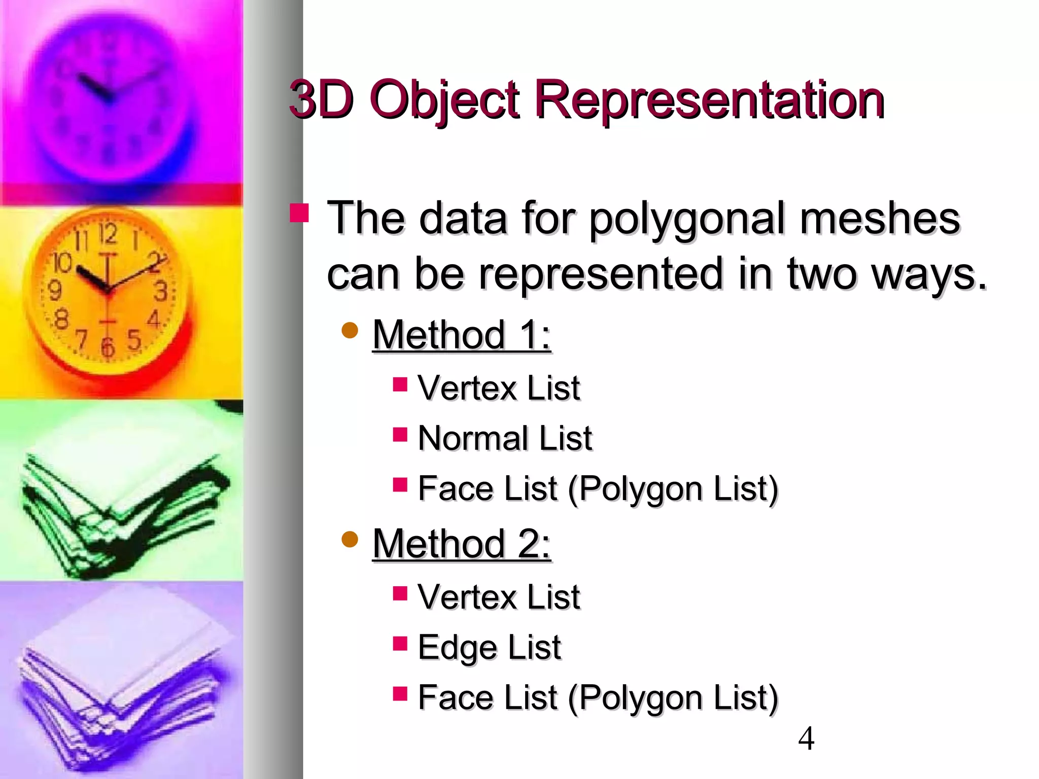
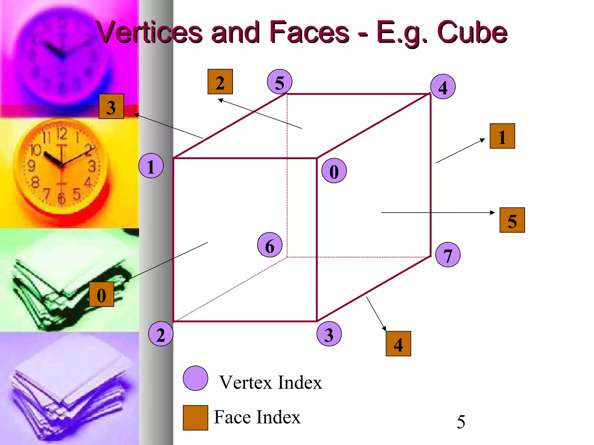
Vertex List Edge List Polygon List
x[i] y[i] z[i] L[j] M[j] P[k] Q[k] R[k] S[k]
30 30 30 0 1 0 1 2 3
-30 30 30 1 2 4 7 6 5
-30 -30 30 2 3 0 4 5 1
30 -30 30 3 0 1 5 6 2
30 30 -30 4 5 2 6 7 3
-30 30 -30 5 6 3 7 4 0
-30 -30 -30 6 7
30 -30 -30 7 4
0 4
1 5
2 6
3 7
Data representation using vertex, face and edge lists:](https://image.slidesharecdn.com/1422798749-151111190641-lva1-app6892/75/1422798749-2779lecture-5-7-2048.jpg)
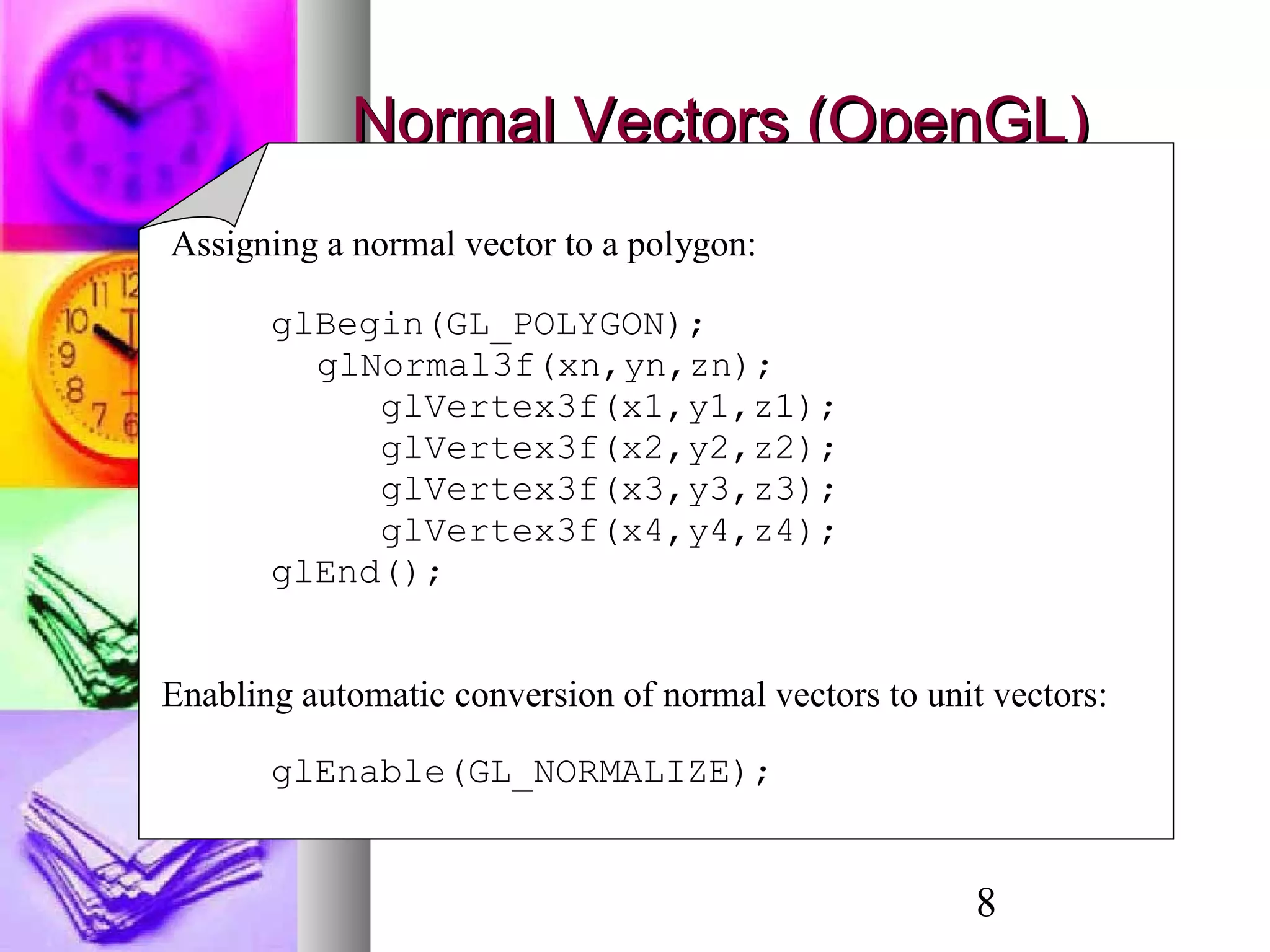


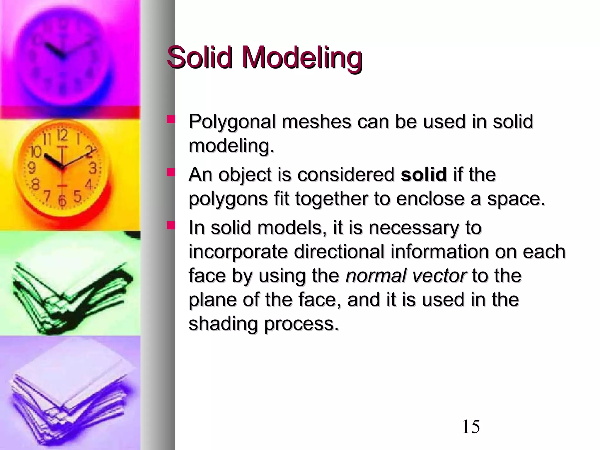
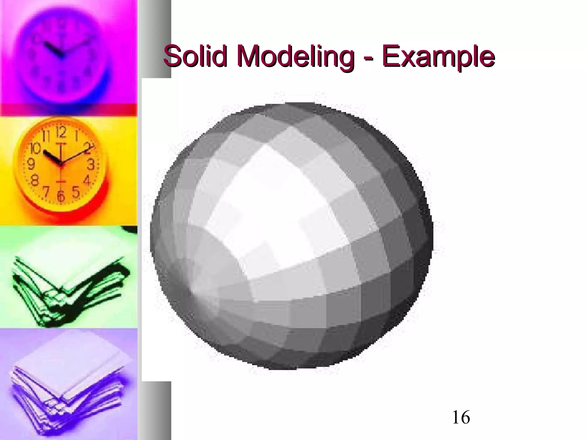
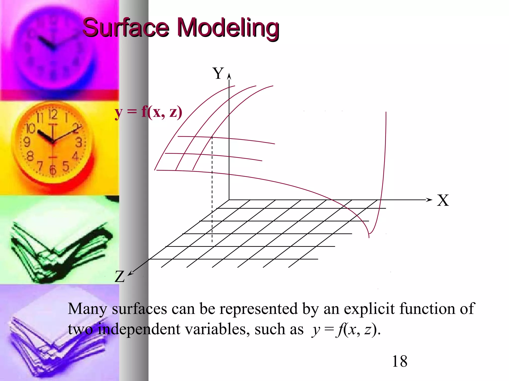
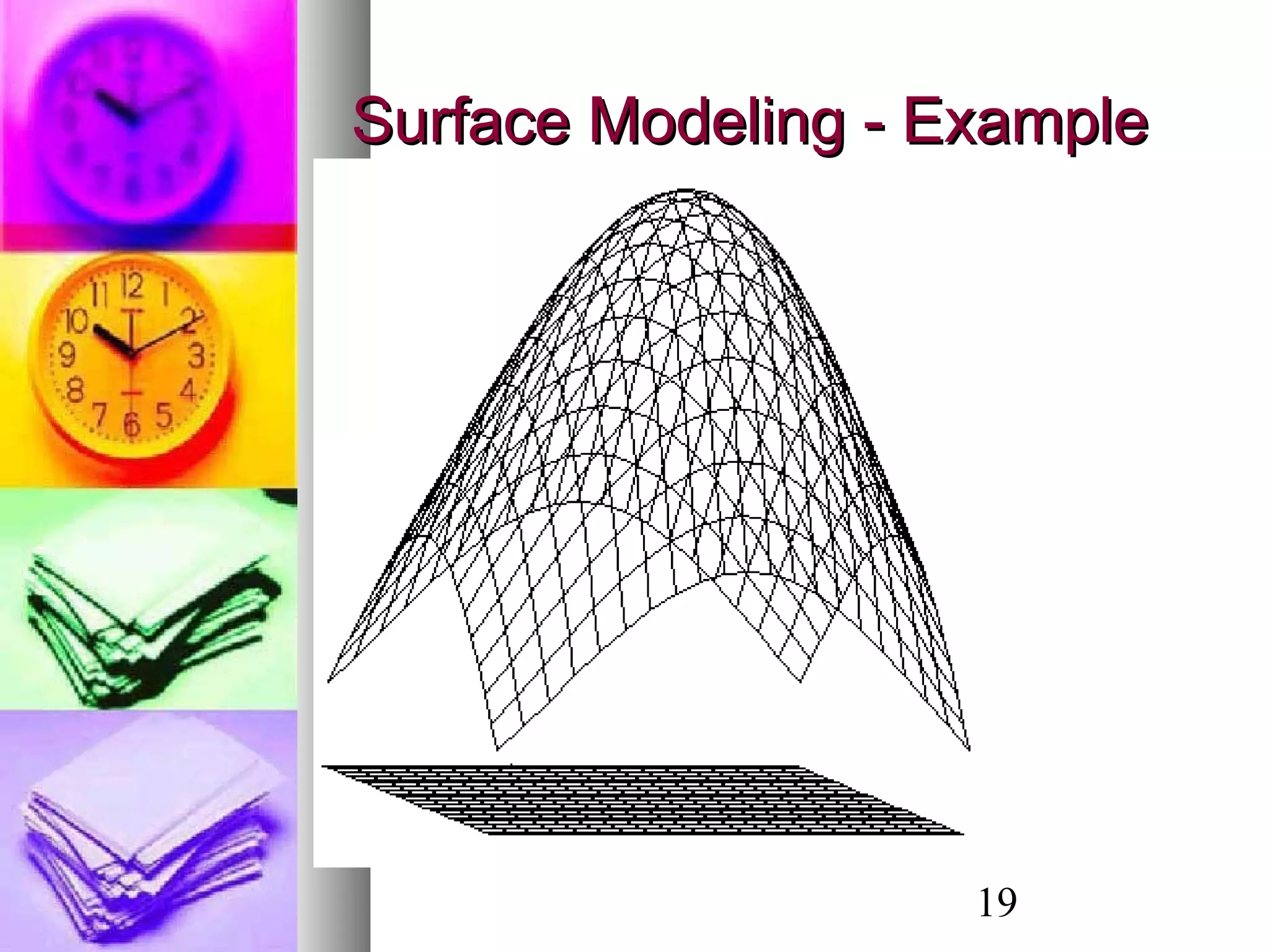

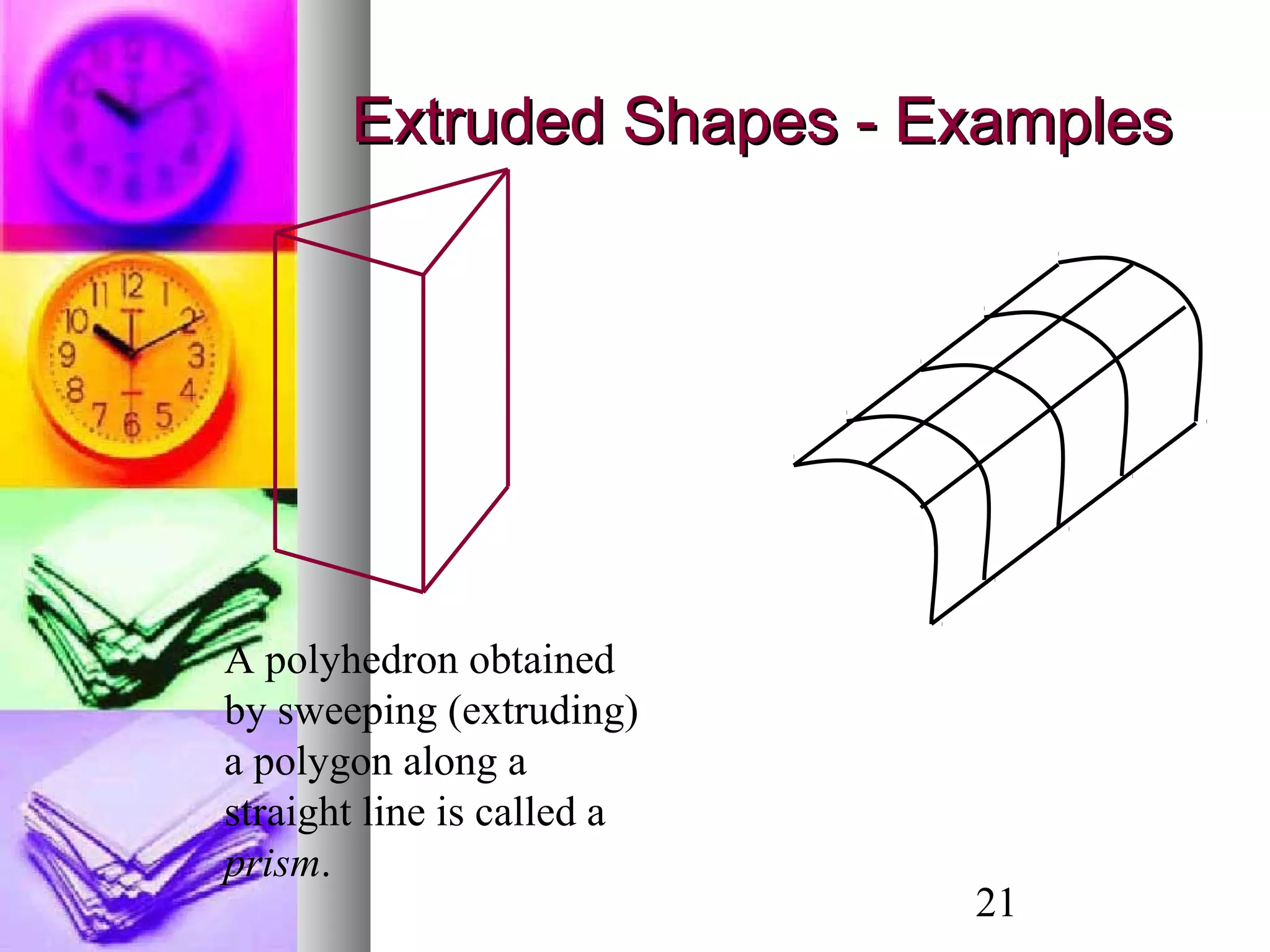
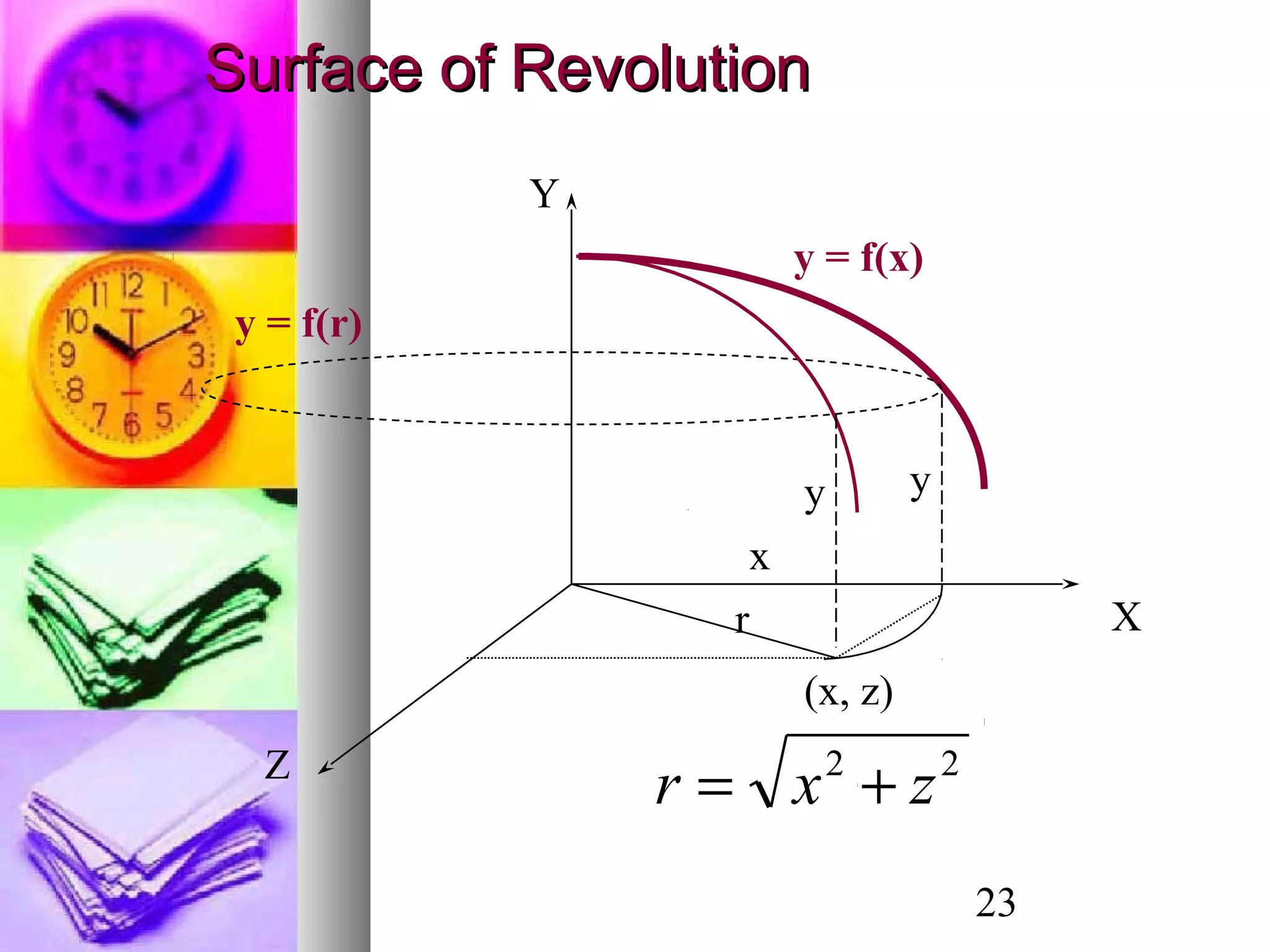

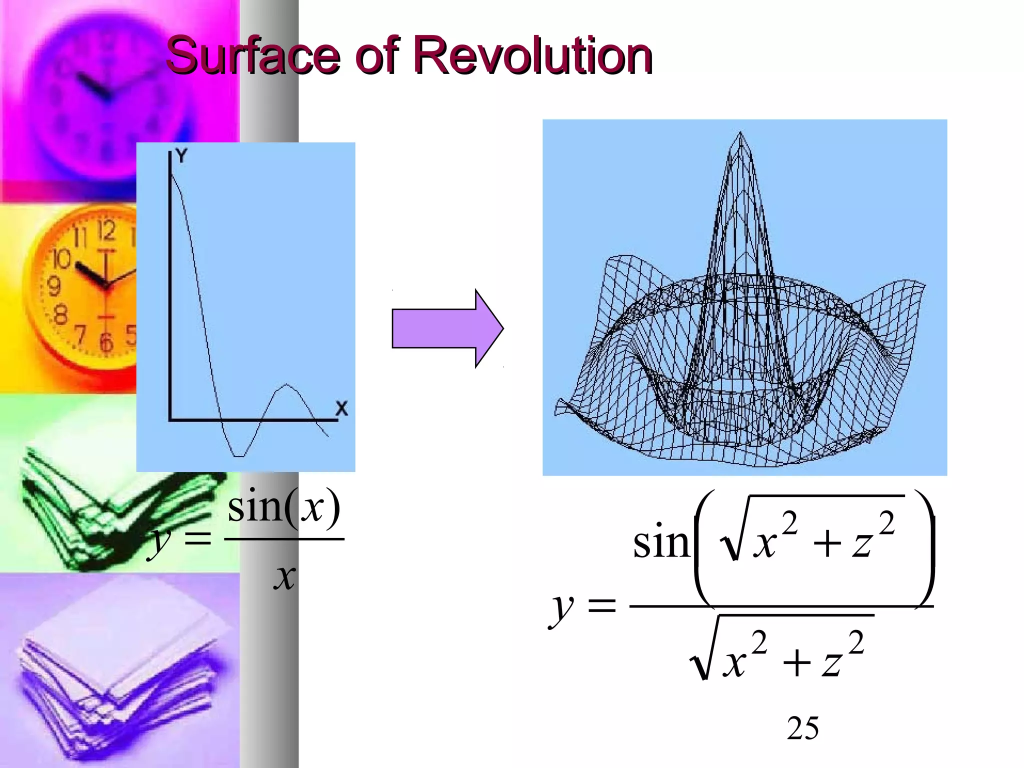


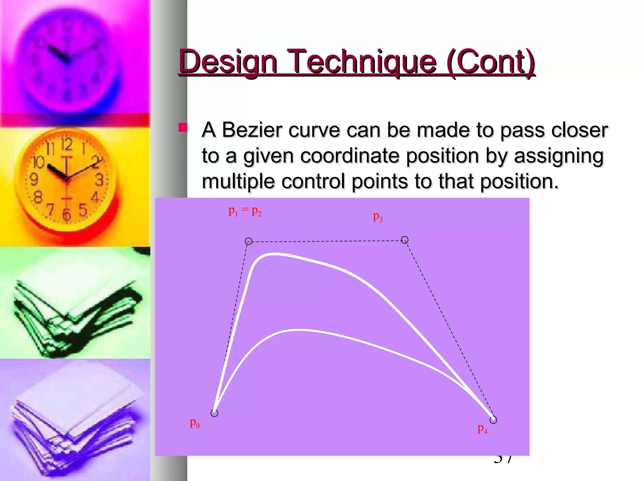
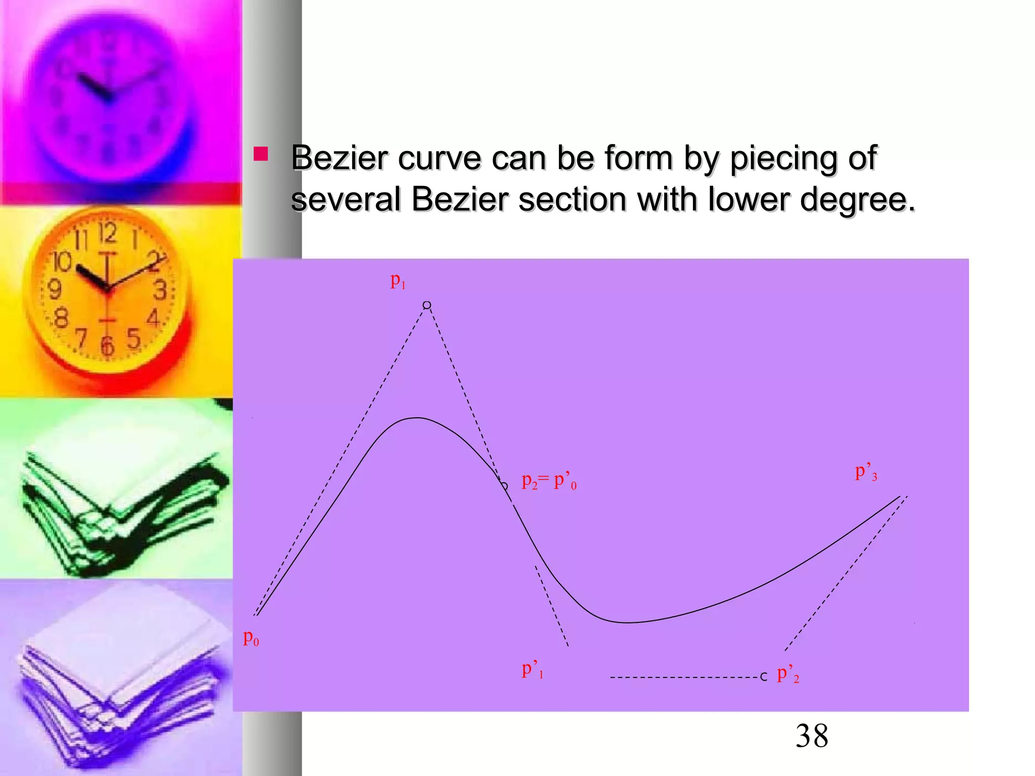

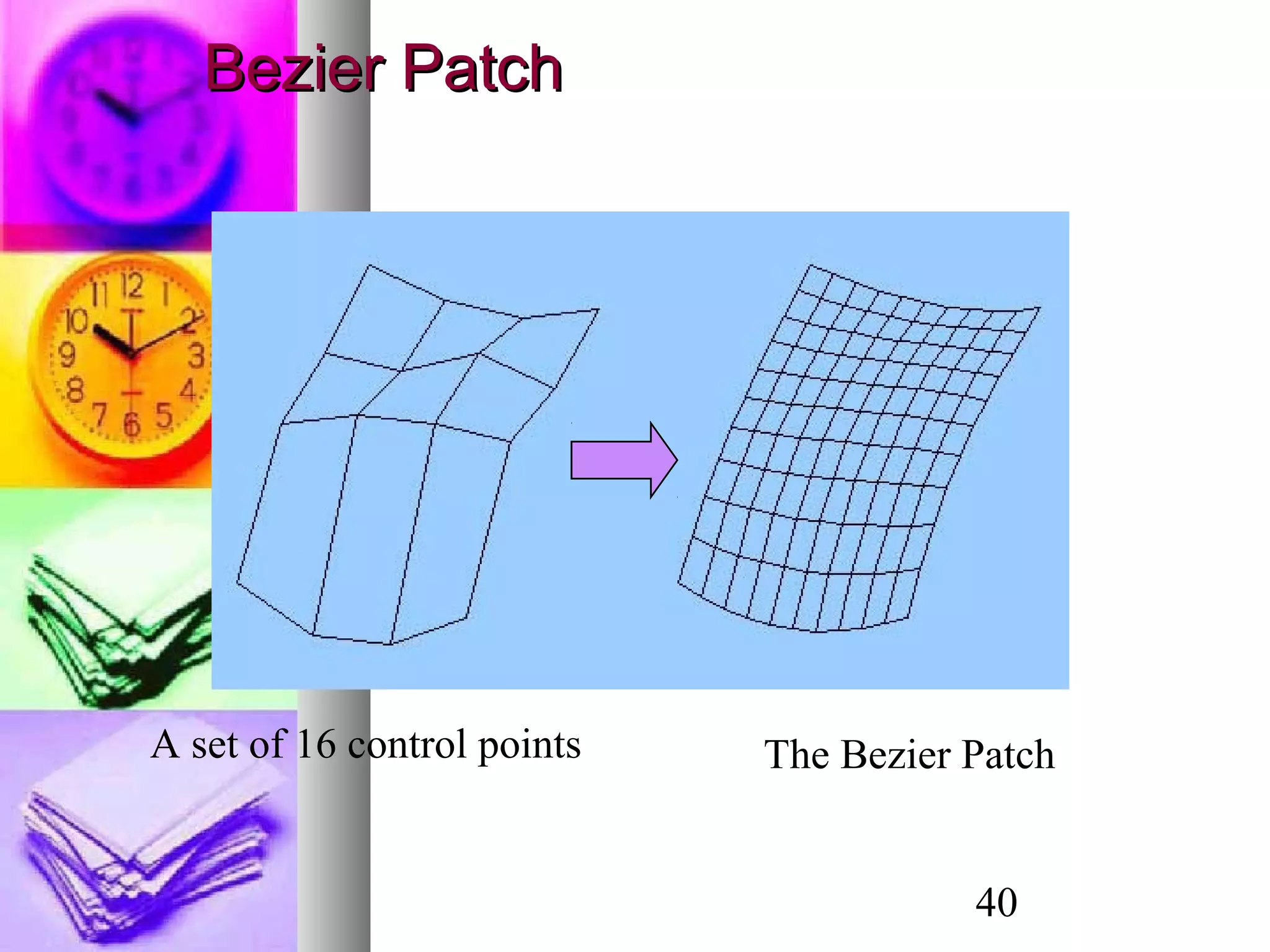


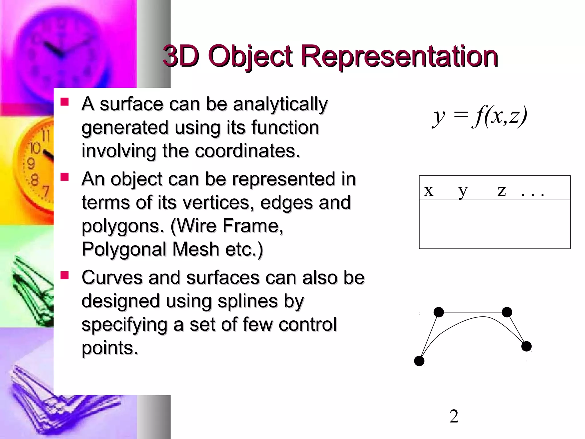
The document discusses various methods for 3D object modeling and representation, including: - Polygonal meshes which approximate surfaces and solids using polygons and can represent a broad class of objects. - Solid modeling using polygonal meshes where directional information is added to faces using normal vectors. - Sweep representations that form shapes by extruding or sweeping 2D profiles through space. - Surface modeling using explicit functions of two variables or surfaces of revolution obtained by rotating curves around axes.


![Solids[1]](https://cdn.slidesharecdn.com/ss_thumbnails/solids1-150926053431-lva1-app6891-thumbnail.jpg?width=640&height=640&fit=bounds)


