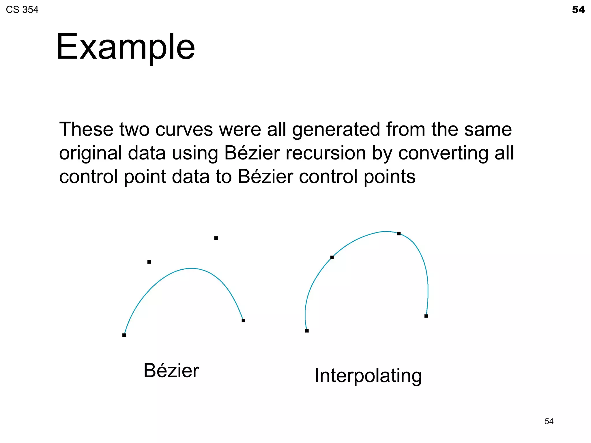
Downloaded 665 times


![CS 354 7
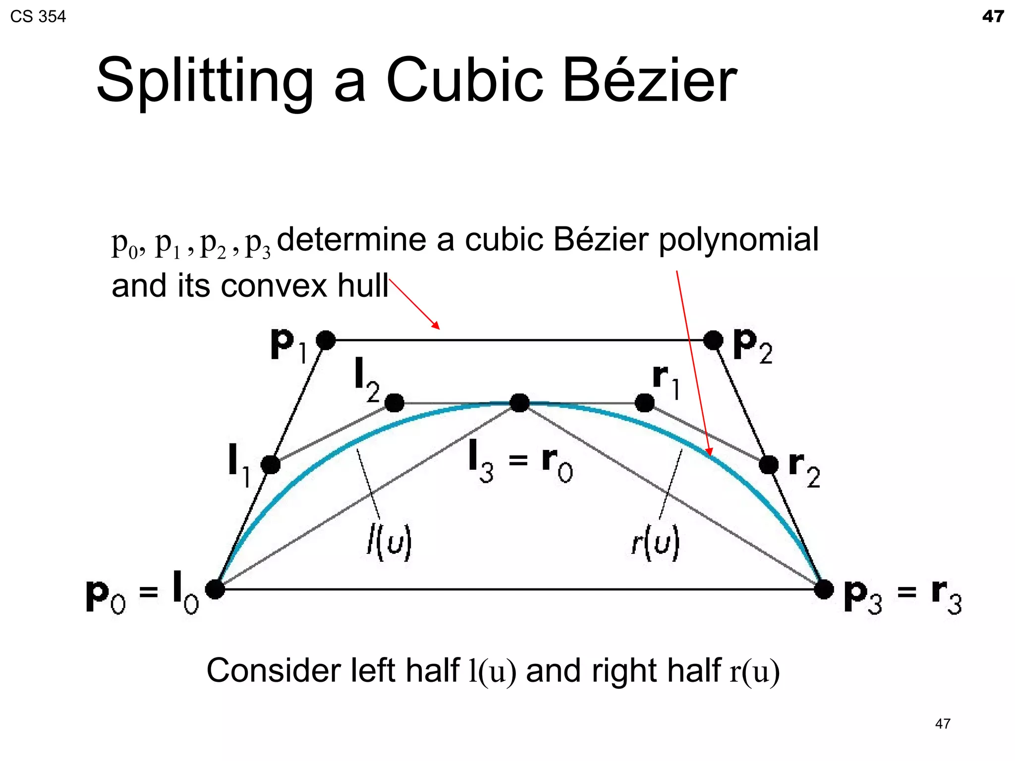
Procedurally Generating a
Torus from a 2D Grid
2D grid over (s,t)∈[0,1]
Tessellated torus](https://image.slidesharecdn.com/21bezier-120408025345-phpapp02/75/CS-354-Bezier-Curves-7-2048.jpg)
![CS 354 11
Coordinate Spaces for Project 2
Parametric space
2D space [0..1]x[0..1] for 2D patch
Object space
Transform the patch’s parametric space into a 3D space
containing a torus
Has modeling transformation from object- to world-space
World space
Environment map is oriented in this space
gluLookAt’s coordinates are in this space
Surface space
(0,0,1) is always surface normal direction
Mapping from object space to surface space varies along torus
Perturbed normal from normal map overrides (0,0,1) geometric
normal
Eye space
gluLookAt transforms world space to eye space](https://image.slidesharecdn.com/21bezier-120408025345-phpapp02/75/CS-354-Bezier-Curves-11-2048.jpg)
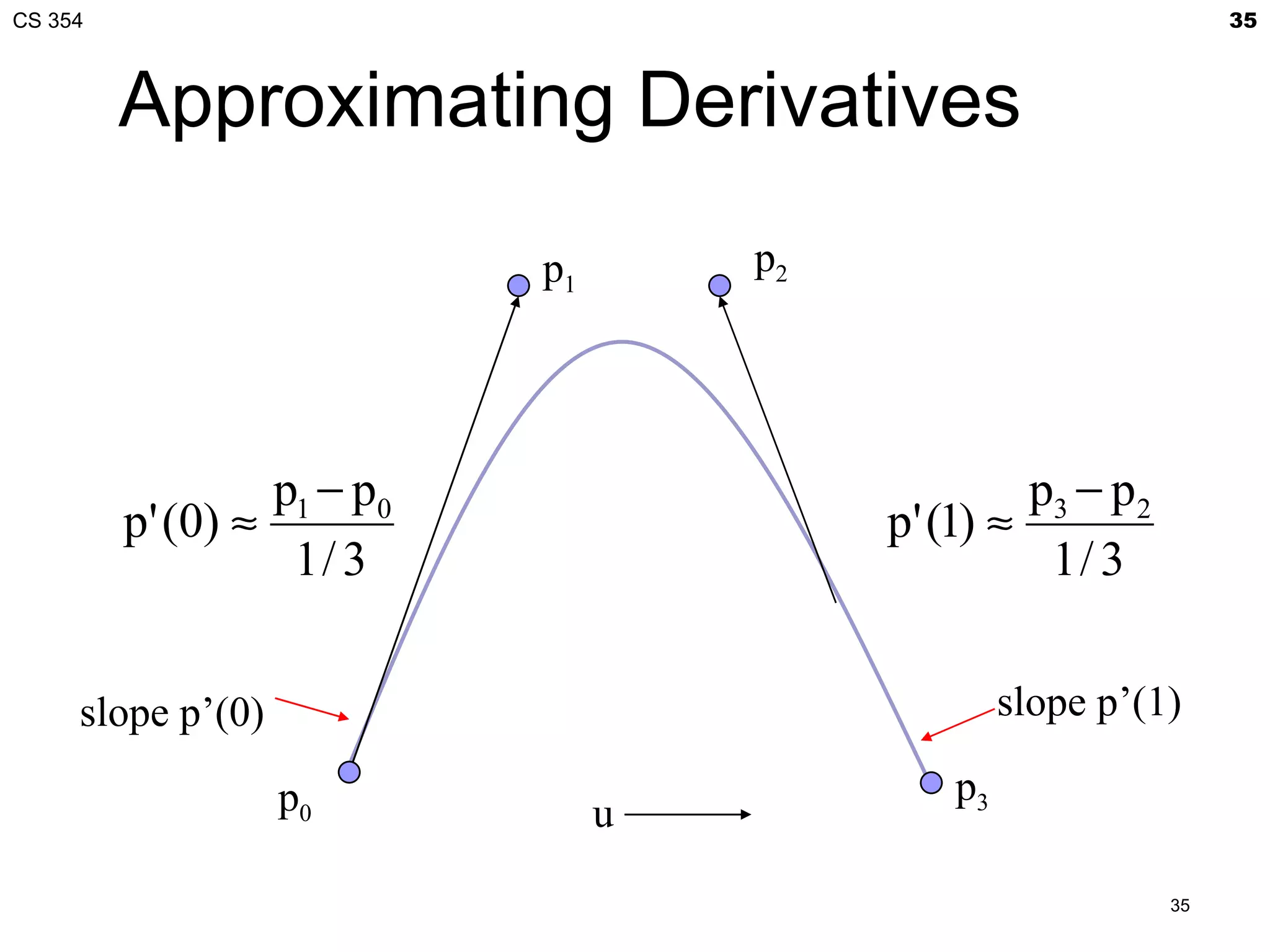
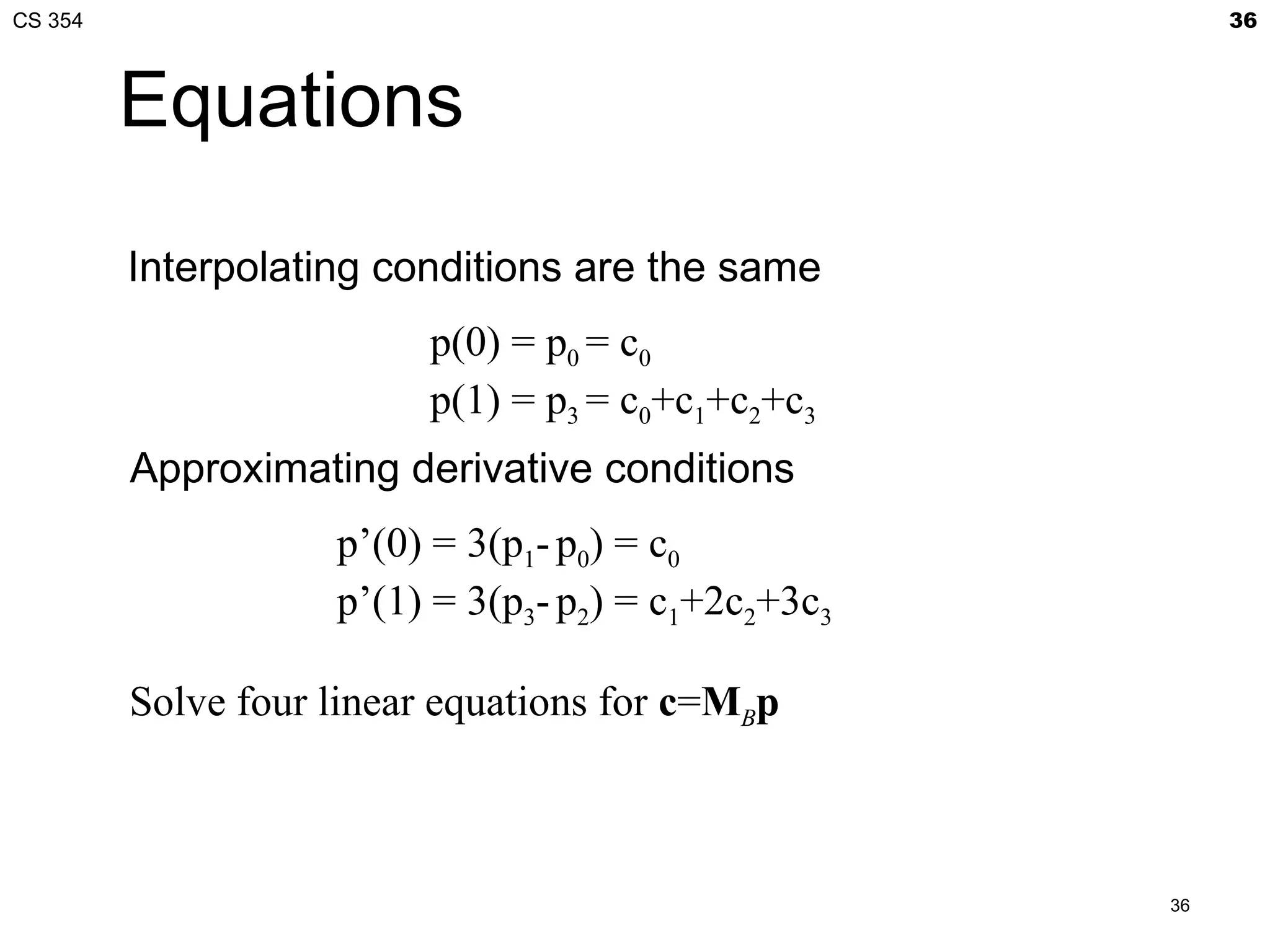
![CS 354 17
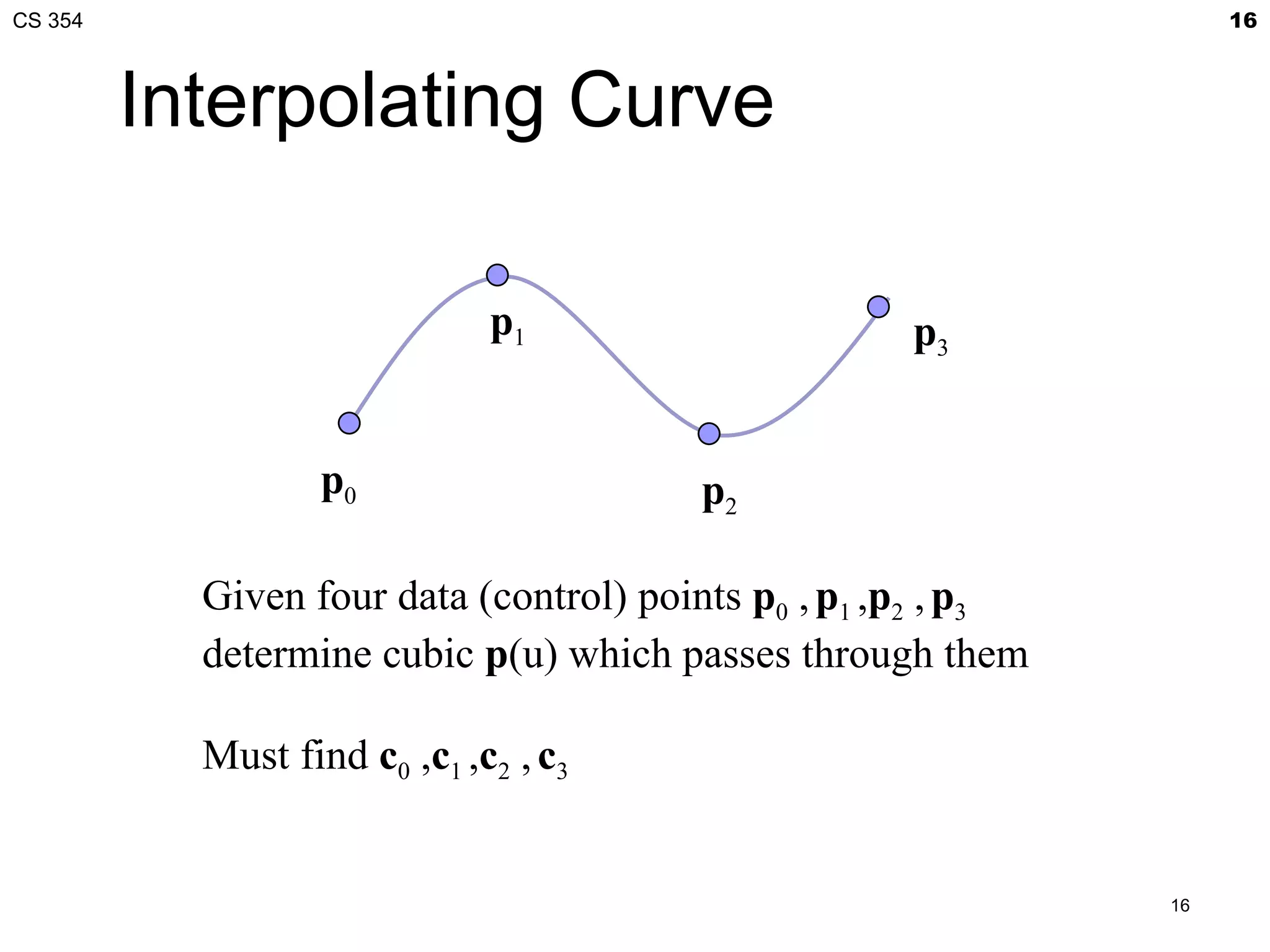
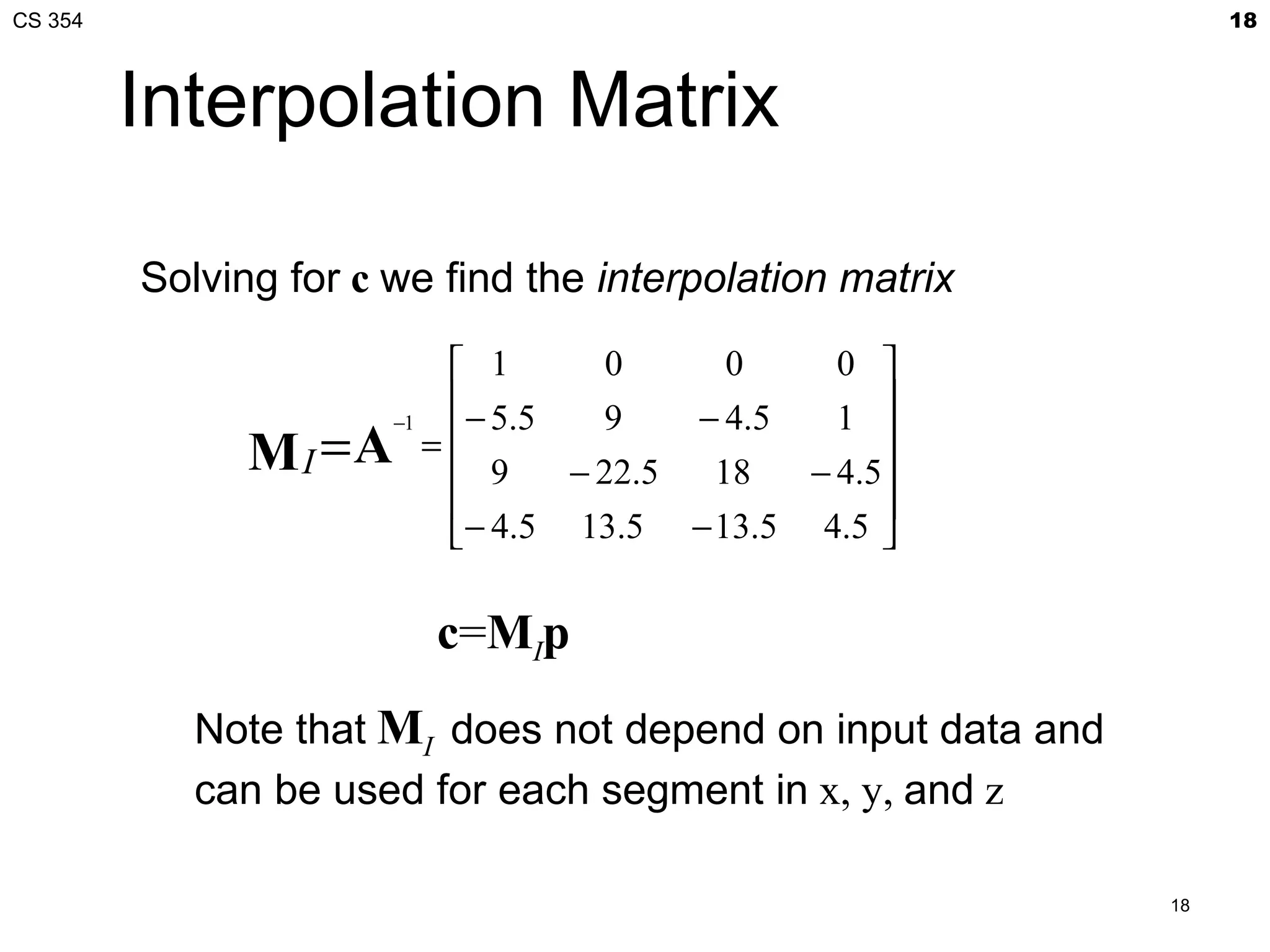
Interpolation Equations
apply the interpolating conditions at u=0, 1/3, 2/3, 1
p0=p(0)=c0
p1=p(1/3)=c0+(1/3)c1+(1/3)2c2+(1/3)3c2
p2=p(2/3)=c0+(2/3)c1+(2/3)2c2+(2/3)3c2
p3=p(1)=c0+c1+c2+c2
or in matrix form with p = [p0 p1 p2 p3]T
1 0 0 0
1 1
2
1
3
1
3 3 3
p=Ac A=
2 2
2
2
3
1
3 3 3
1
1 1 1
17](https://image.slidesharecdn.com/21bezier-120408025345-phpapp02/75/CS-354-Bezier-Curves-17-2048.jpg)
![CS 354 19
Interpolating Multiple
Segments
use p = [p0 p1 p2 p3] T use p = [p3 p4 p5 p6]T
Get continuity at join points but not
continuity of derivatives
19](https://image.slidesharecdn.com/21bezier-120408025345-phpapp02/75/CS-354-Bezier-Curves-19-2048.jpg)
![CS 354 20
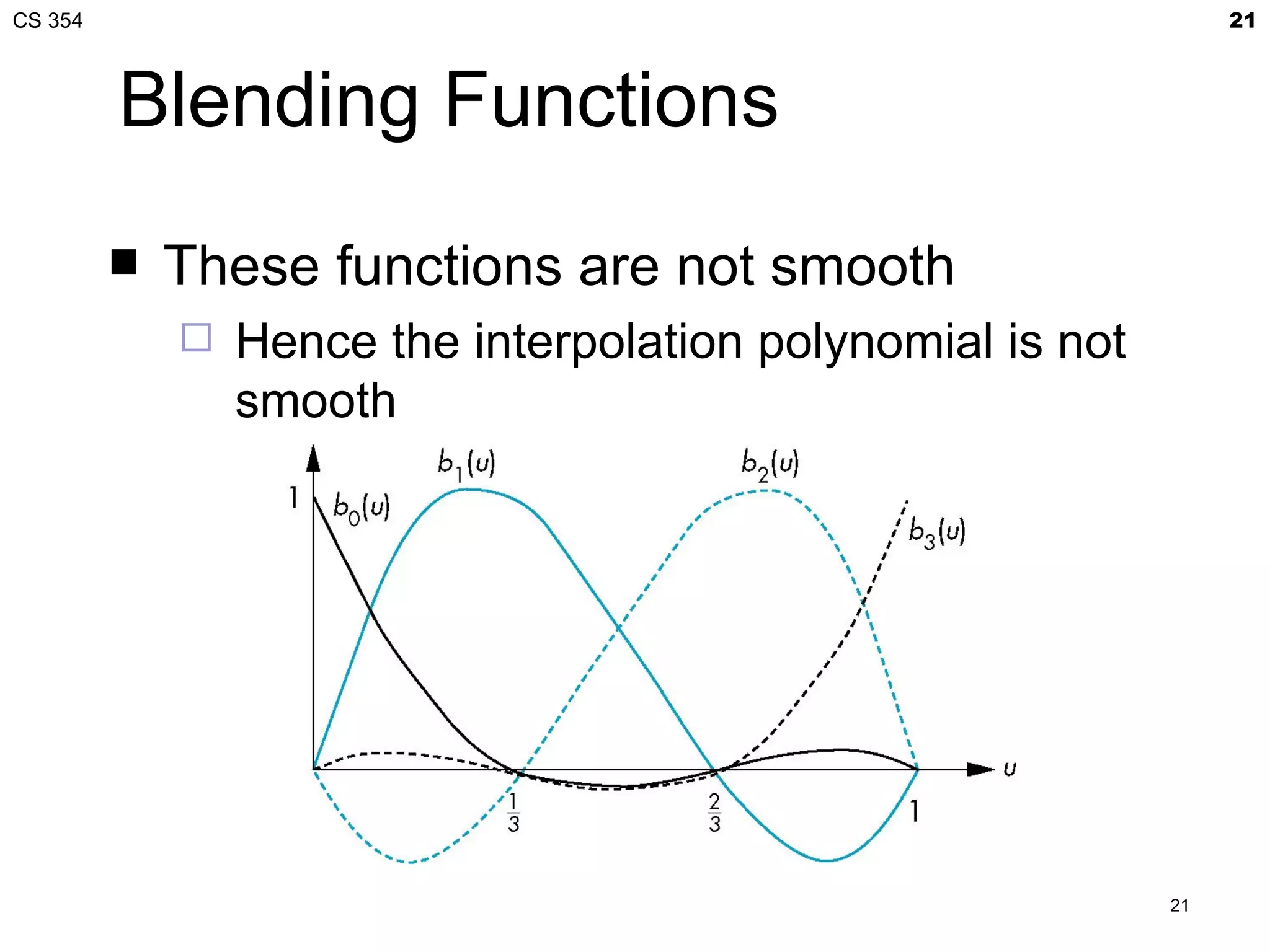
Blending Functions
Rewriting the equation for p(u)
p(u)=uTc=uTMIp = b(u)Tp
where b(u) = [b0(u) b1(u) b2(u) b3(u)]T is
an array of blending polynomials such that
p(u) = b0(u)p0+ b1(u)p1+ b2(u)p2+ b3(u)p3
b0(u) = -4.5(u-1/3)(u-2/3)(u-1)
b1(u) = 13.5u (u-2/3)(u-1)
b2(u) = -13.5u (u-1/3)(u-1)
b3(u) = 4.5u (u-1/3)(u-2/3)
20](https://image.slidesharecdn.com/21bezier-120408025345-phpapp02/75/CS-354-Bezier-Curves-20-2048.jpg)
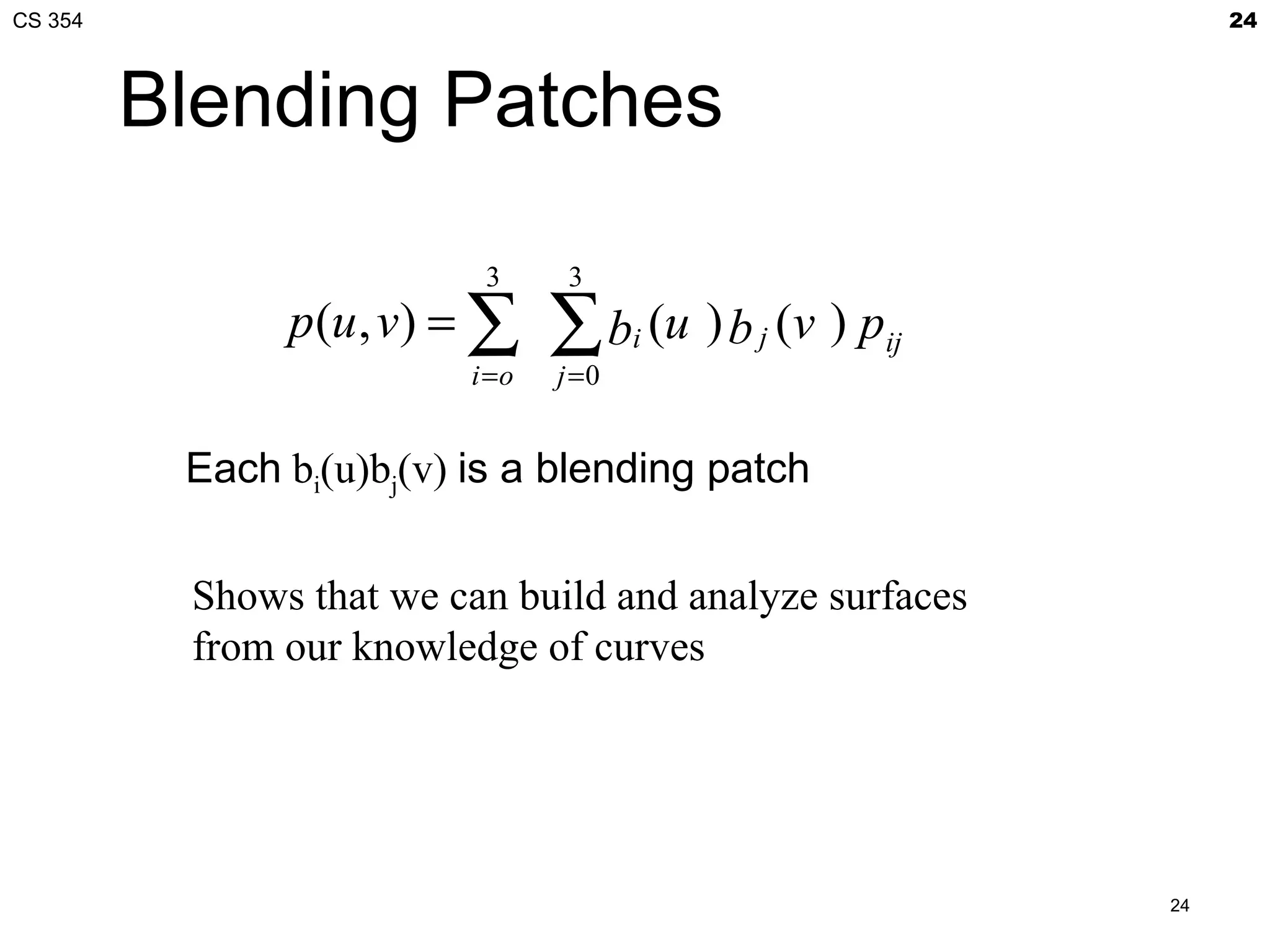
![CS 354 23
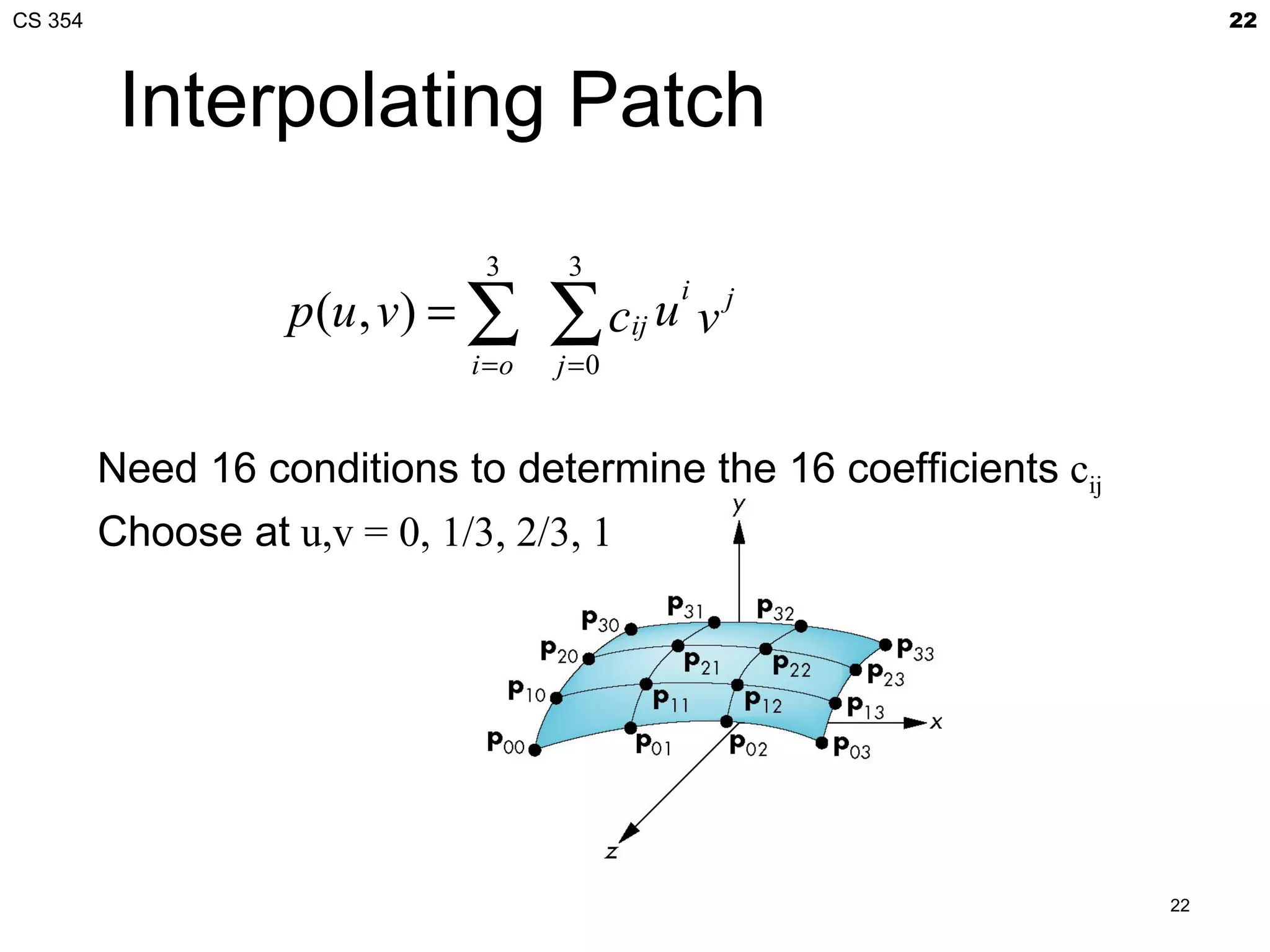
Matrix Form
Define v = [1 v v2 v3]T
C = [cij] P = [pij]
p(u,v) = uTCv
If we observe that for constant u (v), we obtain
interpolating curve in v (u), we can show
C=MIPMI
p(u,v) = uTMIPMITv
23](https://image.slidesharecdn.com/21bezier-120408025345-phpapp02/75/CS-354-Bezier-Curves-23-2048.jpg)

![CS 354 41
Bézier Patches
Using same data array P=[pij] as with interpolating form
3 3
p (u , v) = ∑∑ bi (u ) b j (v) pij = uT M B P MT v
B
i =0 j =0
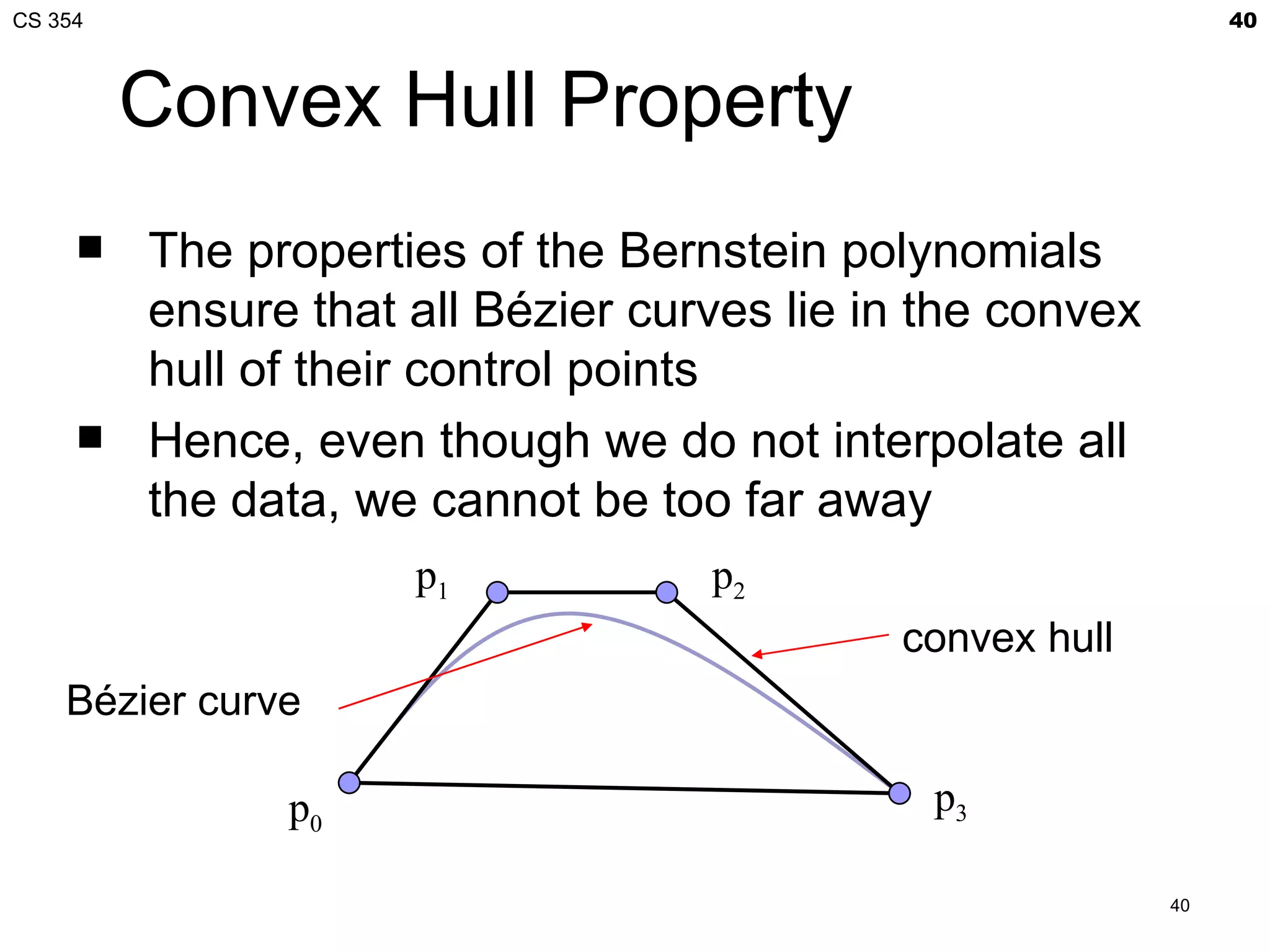
Patch lies in
convex hull
41](https://image.slidesharecdn.com/21bezier-120408025345-phpapp02/75/CS-354-Bezier-Curves-41-2048.jpg)
![CS 354 59
Quadrics
Any quadric can be written as the quadratic form
pTAp+bTp+c=0 where p=[x, y, z]T
with A, b and c giving the coefficients
Render by ray casting
Intersect with parametric ray p(α)=p0+αd that
passes through a pixel
Yields a scalar quadratic equation
No solution: ray misses quadric
One solution: ray tangent to quadric
Two solutions: entry and exit points
59](https://image.slidesharecdn.com/21bezier-120408025345-phpapp02/75/CS-354-Bezier-Curves-59-2048.jpg)

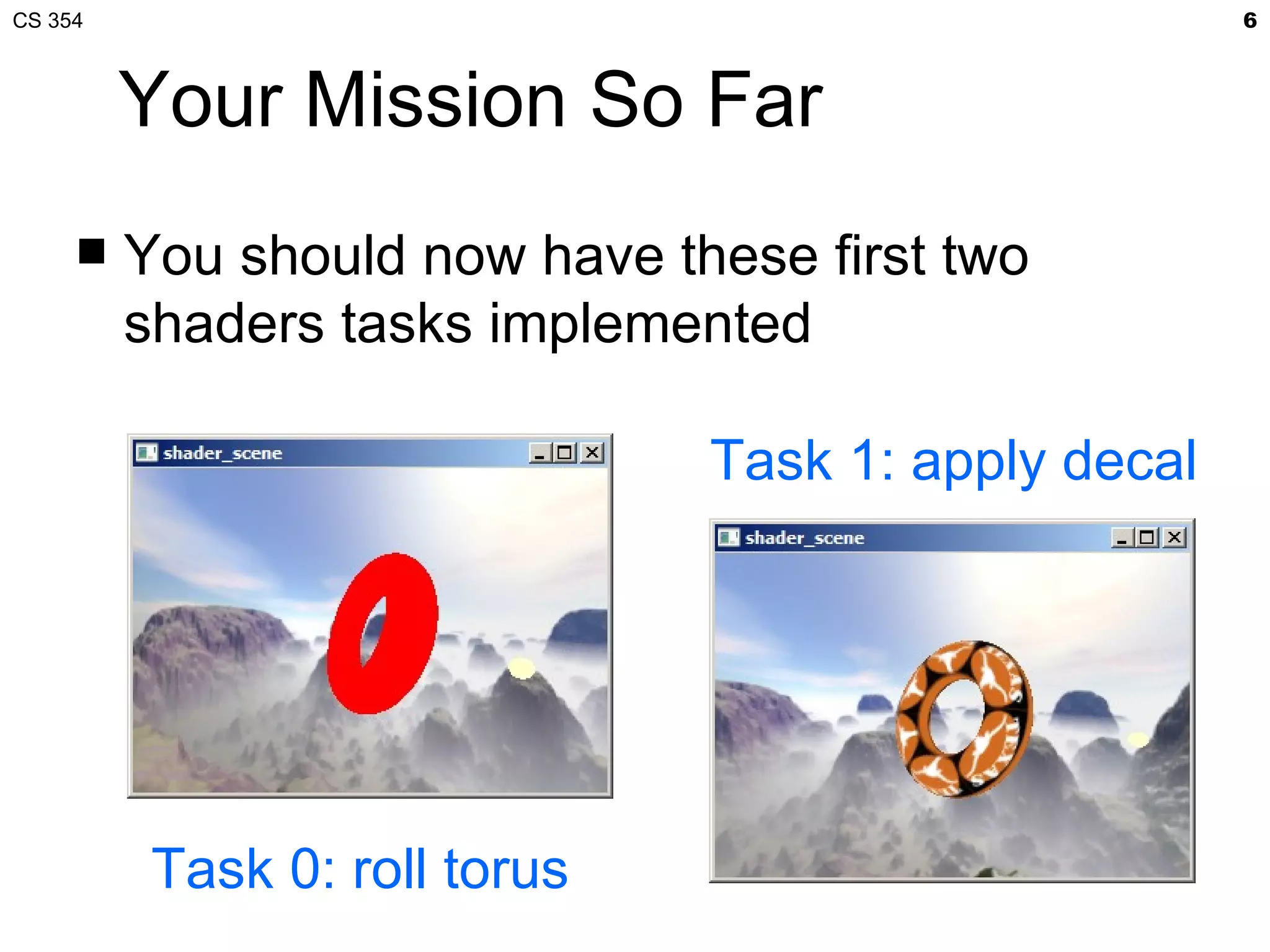
The document discusses Bézier curves and provides information about a CS 354 class. It includes details about an in-class quiz, the professor's office hours, and an upcoming lecture on Bézier curves and Project 2, which is due on Friday. The lecture will cover procedural generation of a torus from a 2D grid, GLSL functions needed for the project, normal maps, coordinate spaces, interpolation curves, and Bézier curves.