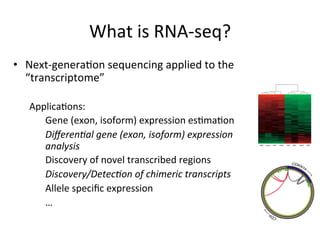
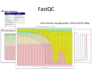
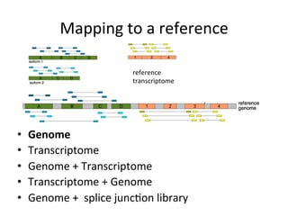
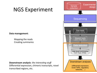
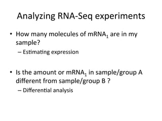
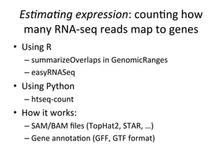
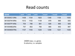
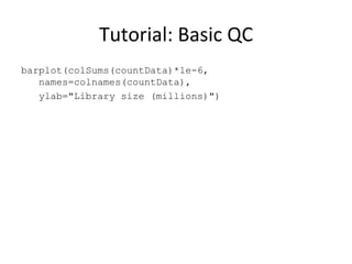
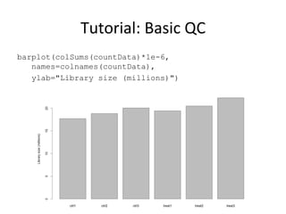
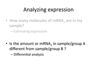
This document provides an overview of RNA-seq data analysis. It discusses quality control of sequencing data using tools like FastQC, mapping reads to a reference genome or transcriptome using aligners like BWA and TopHat, and summarizing reads using counting tools to obtain read counts for each gene. These counts can then be used to estimate gene expression levels and perform differential expression analysis to identify genes with different expression between samples or conditions.

![QC
and
pre-‐processing
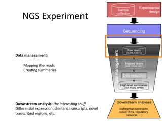
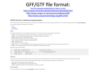
• First
step
in
QC:
– Look
at
quality
scores
to
see
if
sequencing
was
successful
• Sequence
data
usually
stored
in
FASTQ
format:
@BI:080831_SL-XAN_0004_30BV1AAXX:8:1:731:1429#0/1
GTTTCAACGGGTGTTGGAATCCACACCAAACAATGGCTACCTCTATCACCC
+
hbhhP_Z[`VFhHNU]KTWPHHIKMIIJKDJGGJGEDECDCGCABEAFEB
Header
(typically
w/
flowcell
#)
Sequence
Quality
scores
flow
cell
lane
Cle
number
x-‐coordinate
y-‐coordinate
provided
by
user
1st
end
of
paired
read
40,34,40,40,16,31,26,28,27,32,22,6,40,8,14,21,29,11,20,23,16,…
ASCII
table
Numerical
quality
scores
Typical
range
of
quality
scores:
0
~
40](https://image.slidesharecdn.com/lecture20sboner-240405072050-d16a7392/85/RNA-sequencing-analysis-tutorial-with-NGS-5-320.jpg)


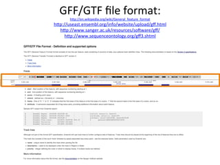
![Tutorial:
Installing
BioConductor
packages
source("http://bioconductor.org/biocLite.R")
biocLite("DESeq2")
hep://www.bioconductor.org/
M.
I.
Love,
W.
Huber,
S.
Anders:
Moderated
esCmaCon
of
fold
change
and
dispersion
for
RNA-‐Seq
data
with
DESeq2.
bioRxiv
(2014).
doi:
10.1101/002832
[1]](https://image.slidesharecdn.com/lecture20sboner-240405072050-d16a7392/85/RNA-sequencing-analysis-tutorial-with-NGS-26-320.jpg)
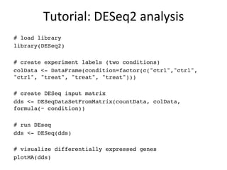
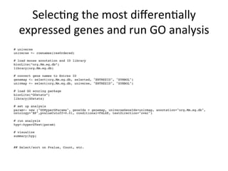
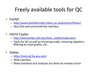
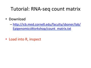
![Tutorial:
DESeq2
analysis
# load library
library(DESeq2)
# create experiment labels (two conditions)
colData <- DataFrame(condition=factor(c("ctrl","ctrl", "ctrl", "treat", "treat", "treat")))
# create DESeq input matrix
dds <- DESeqDataSetFromMatrix(countData, colData, formula(~ condition))
# run DEseq
dds <- DESeq(dds)
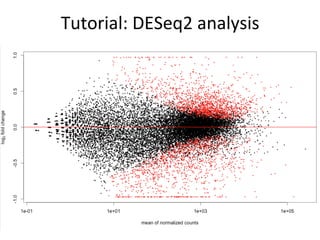
# visualize differentially expressed genes
plotMA(dds)
# get differentially expressed genes
res <- results(dds)
# order by BH adjusted p-value
resOrdered <- res[order(res$padj),]
# top of ordered matrix
head(resOrdered)](https://image.slidesharecdn.com/lecture20sboner-240405072050-d16a7392/85/RNA-sequencing-analysis-tutorial-with-NGS-29-320.jpg)
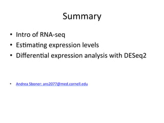
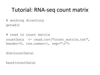
![Tutorial:
DESeq2
analysis
# get differentially expressed genes
res <- results(dds)
# order by BH adjusted p-value
resOrdered <- res[order(res$padj),]
# top of ordered matrix
head(resOrdered)
DataFrame with 6 rows and 6 columns
baseMean log2FoldChange lfcSE stat pvalue padj
<numeric> <numeric> <numeric> <numeric> <numeric> <numeric>
Pck1 19300.0081 -2.3329116 0.16519373 -14.12228 2.768978e-45 3.986497e-41
Fras1 1202.1842 -0.8469410 0.06499738 -13.03039 8.219001e-39 5.916448e-35
S100a14 590.6305 2.1903041 0.17608923 12.43860 1.612985e-35 7.740716e-32
Ugt1a2 2759.7012 -1.7037495 0.15339576 -11.10689 1.161372e-28 4.180067e-25
Crip1 681.0106 0.7717364 0.07264577 10.62328 2.322502e-26 5.572844e-23
Smpdl3a 11152.4458 0.3398371 0.03195000 10.63653 2.014913e-26 5.572844e-23
# how many differentially expressed genes ? FDR=10%, |fold-change|>2 (up and down)](https://image.slidesharecdn.com/lecture20sboner-240405072050-d16a7392/85/RNA-sequencing-analysis-tutorial-with-NGS-30-320.jpg)
![Tutorial:
DESeq2
analysis
# how many differentially expressed genes ? FDR=10%, |fold-change|>2 (up and down)
# get differentially expressed gene matrix
sig <- resOrdered[!is.na(resOrdered$padj) &
resOrdered$padj<0.10 &
abs(resOrdered$log2FoldChange)>=1,]](https://image.slidesharecdn.com/lecture20sboner-240405072050-d16a7392/85/RNA-sequencing-analysis-tutorial-with-NGS-31-320.jpg)
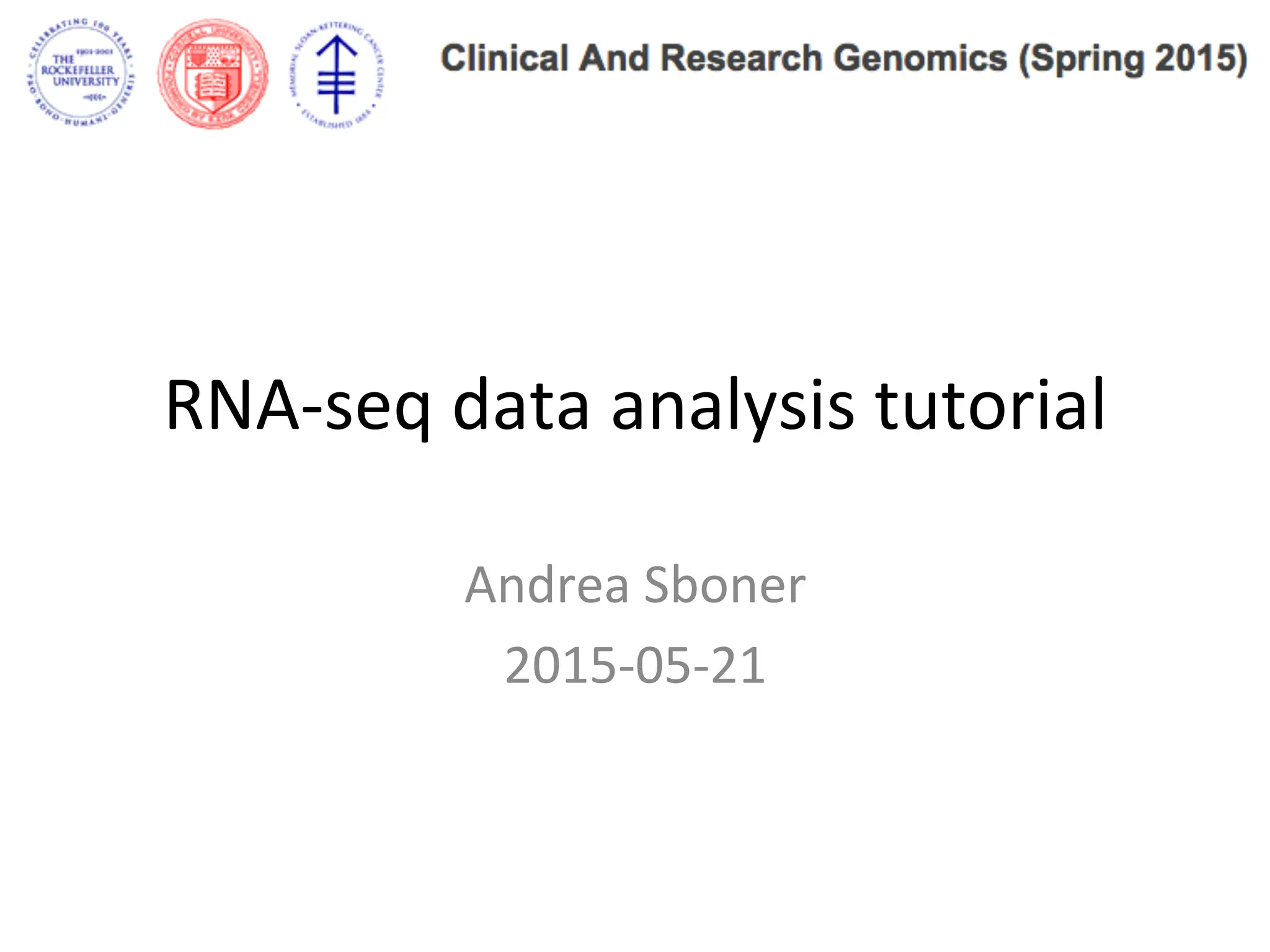
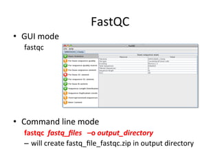
![Tutorial:
DESeq2
analysis
# how many differentially expressed genes ? FDR=10%, |fold-change|>2 (up and down)
# get differentially expressed gene matrix
sig <- resOrdered[!is.na(resOrdered$padj) &
resOrdered$padj<0.10 &
abs(resOrdered$log2FoldChange)>=1,]
head(sig)
DataFrame with 6 rows and 6 columns
baseMean log2FoldChange lfcSE stat pvalue padj
<numeric> <numeric> <numeric> <numeric> <numeric> <numeric>
Pck1 19300 -2.33 0.165 -14.12 2.77e-45 3.99e-41
S100a14 591 2.19 0.176 12.44 1.61e-35 7.74e-32
Ugt1a2 2760 -1.70 0.153 -11.11 1.16e-28 4.18e-25
Pklr 787 -1.00 0.097 -10.34 4.62e-25 9.49e-22
Mlph 1321 1.20 0.117 10.20 1.90e-24 3.42e-21
Ifit1 285 1.39 0.156 8.94 3.76e-19 3.38e-16
dim(sig)
# how to create a heat map](https://image.slidesharecdn.com/lecture20sboner-240405072050-d16a7392/85/RNA-sequencing-analysis-tutorial-with-NGS-32-320.jpg)
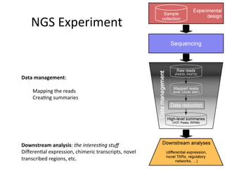
![Tutorial:
Heat
Map
# how to create a heat map
# select genes
selected <- rownames(sig);selected
## load libraries for the heat map
library("RColorBrewer")
source("http://bioconductor.org/biocLite.R")
biocLite(”gplots”)
library("gplots")
# colors of the heat map
hmcol <- colorRampPalette(brewer.pal(9, "GnBu"))(100) ## hmcol <- heat.colors
heatmap.2( log2(counts(dds,normalized=TRUE)[rownames(dds) %in% selected,]),
col = hmcol, scale="row”,
Rowv = TRUE, Colv = FALSE,
dendrogram="row",
trace="none",
margin=c(4,6), cexRow=0.5, cexCol=1, keysize=1 )](https://image.slidesharecdn.com/lecture20sboner-240405072050-d16a7392/85/RNA-sequencing-analysis-tutorial-with-NGS-33-320.jpg)
![Tutorial:
Heat
Map
# how to create a heat map
library("RColorBrewer")
library("gplots")
# colors of the heat map
hmcol <- colorRampPalette(brewer.pal(9, "GnBu"))(100) ## hmcol <- heat.colors
heatmap.2(log2(counts(dds,normalized=TRUE)[rownames(dds) %in% selected,]),
col = hmcol, Rowv = TRUE, Colv = FALSE, scale="row", dendrogram="row", trace="none",
margin=c(4,6), cexRow=0.5, cexCol=1, keysize=1 )](https://image.slidesharecdn.com/lecture20sboner-240405072050-d16a7392/85/RNA-sequencing-analysis-tutorial-with-NGS-34-320.jpg)