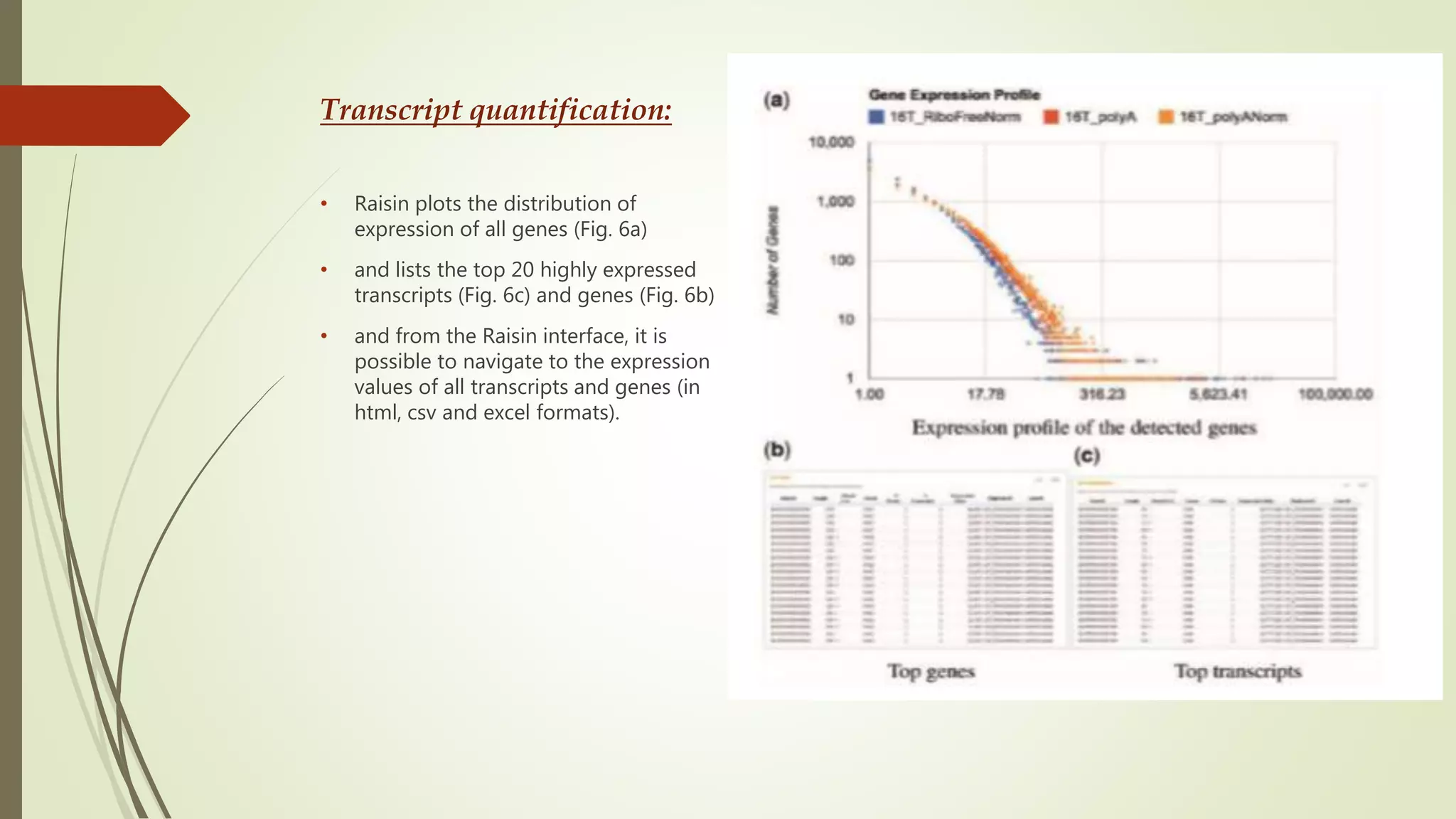
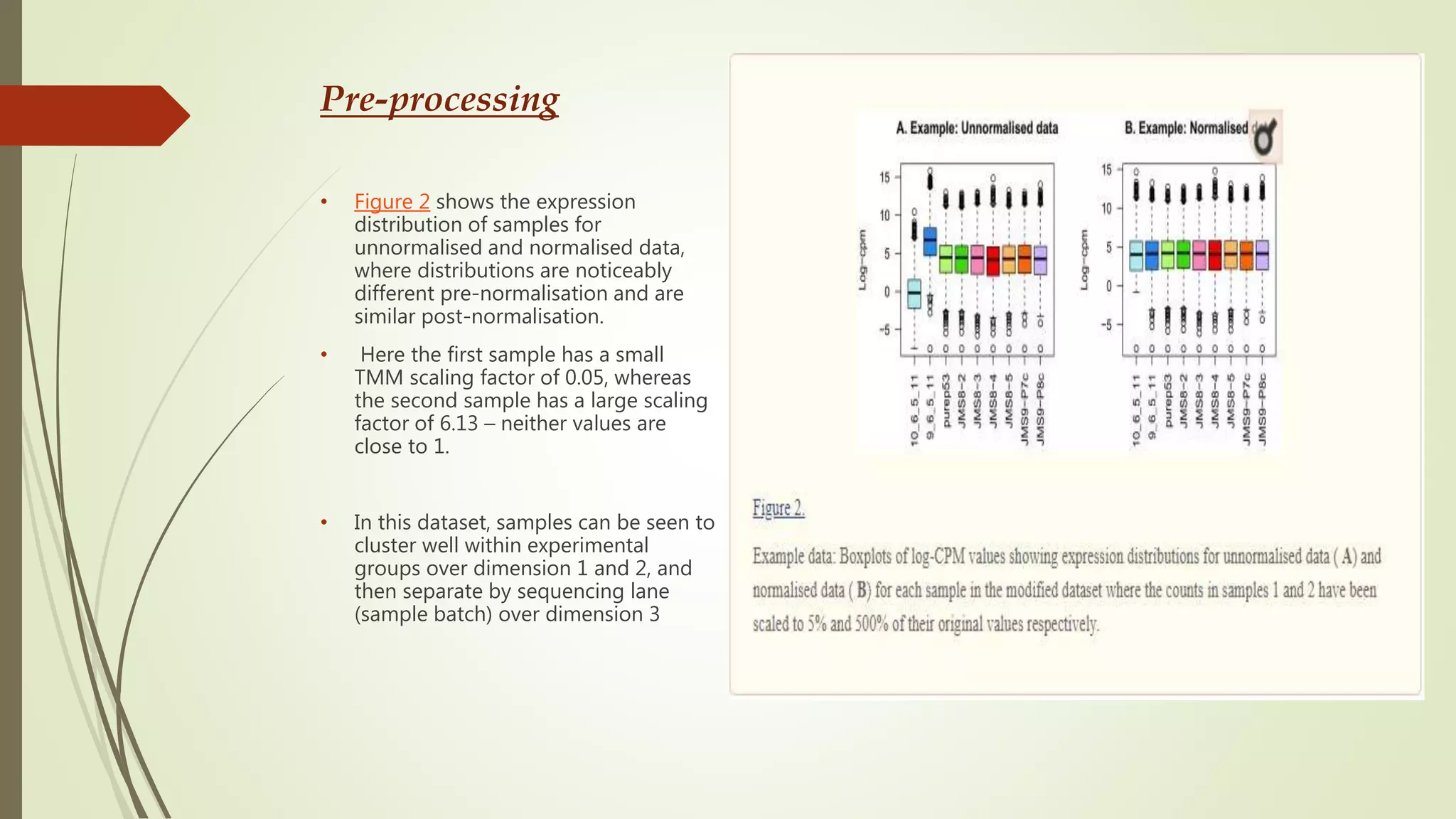
Bioinformatics
 The ability to easily and efficiently analyse RNA-sequencing data is a key strength
of the Bioconductor project
 The development of ultrasequencing technologies during the recent years has
started a major revolution in Biology.
 The ability to directly survey the cell’s RNA content by applying NGS technologies
to cDNA sequencing (‘RNA-Seq’) has provided insights of unprecedented depth on
the transcription landscape of many species such as Homo sapiens.
What is RNA?
 Ribonucleic acid (RNA) is a polymeric molecule essential in various biological
roles in coding, decoding, regulation, and expression of genes
 RNA-Seq (RNA sequencing), also called whole transcriptome shotgun
sequencing(WTSS) , uses next-generation sequencing (NGS) to reveal the
presence and quantity of RNA in a biological sample at a given moment
 RNA-Seq has proven particularly powerful on tasks such as identifying novel
and novel splice forms, detecting low abundance transcripts and finding
variations, such as SNPs
first solution:
Grape RNA-Seq analysis pipeline
 The avalanche of data arriving since the development of NGS (Next-Generation
Sequencing) technologies have prompted the need for developing fast, accurate
and easily automated bioinformatics tools capable of dealing with massive
datasets.
 Among the most productive applications of NGS technologies is the sequencing
of cellular RNA, known as RNA-Seq.
 the lack of standard and user-friendly pipelines is a bottleneck preventing RNA-
Seq from becoming the standard for transcriptome analysis.
 In the specific case of RNA-Seq, mapping of reads is only the first step of a
complex data processing schema, the final goal of which is to produce accurate
gene and transcript quantifications, and to delineate novel transcript structures.
Grape description :
 Grape is an automated workflow integrating the management, analysis and
visualization of RNA-Seq data.
 GRAPE can map the reads to the genome and/or transcriptome, and it can also
work with single or paired end reads, both stranded or not.
Analysis implemented in Grape :
 The main steps in the Grape analysis are as follows:
1. Preprocessing and quality checks
2. Mapping
3. Post-mapping
4. Transcript quantification
5. Discovery and delineation of novel transcribed elements
6. Summary statistics
Preprocessing and quality checks :
 Before processing the reads, Grape creates a number of files and database tables
required for performing the analyses and storing the results.
 Experiments are organized according to the metadata given in the Buildout
configuration files. Next, Grape produces some basic statistics, and checks the
quality of the RNA-Seq data .
Preprocessing and
quality checks:
• Figures 2 a, b and d illustrate the
Raisin interface to some of these QC
steps.
• These initial QC steps contribute to
assess whether additional
preprocessing, such as trimming
and/or filtering of the reads, is
necessary.
• However, Grape only provides the QC
information, and it is up to the user to
decide whether additional
preprocessing is required .
Mapping :
 Grape’s next step is the alignment of the short sequence reads to the reference
genome. This step is crucial for the RNA-Seq analysis, as it will condition any
downstream analyses.
 when examining transcriptome data, reads mapping across splice junctions will not
match the genome sequence, and it is convenient to create a specific index
corresponding to the splice junctions.
 Junction mappings are filtered to remove those reads that do not span the splice
site. Next, the remaining unmapped reads are mapped using the GEM split-
mapper.
Mapping :
• For each number of mismatches, a
new genome mapping (including
split-mapping) is performed.
• Second, remaining unmapped reads
are successively trimmed by a set
number of nucleotides (10 by default),
and a new genome (and split)
mapping performed after each
trimming.
• This iterative mapping ends when all
reads are mapped, or the length of
the reads falls below a certain
threshold.
Post-mapping :
 The reads that align in the initial round of mapping (genome, junction and split-
mapping) are examined and divided into those reads that map to one location
better than to any other (unique map).
 The eventual use of one read alignment type versus the other will depend on the
type of the analysis.
 For example, for tasks such as the identification of novel genes, or the detection of
low abundance transcripts, the confidence of the results increases if only uniquely
mapped reads are considered. Other tasks, like the calculation of
genome/transcriptome coverage, may use all the mapped reads.
Post-mapping:
• Figure4 Raisin visualization of Grape’s
mapping step.
• Panel a shows the overall mapping
results as well as the information on the
genome annotation and number of
mismatches used for the alignments.
• Panel b shows the fraction of reads
aligned in the final merged mapping.
• Panels c, d and e show the same type of
information for the different components
of the mapping process
• The results of the different mapping steps
are combined into a final mapping results
file in GFF, BED or SAM/BAM format
Transcript quantification :
 Grape uses the mapping results to produce quantifications of the abundance of a
number of transcribed elements: exons, splice junctions, genes and transcripts, as
well as inclusion indices for exons.
 To produce quantifications of individual transcripts, we use the FluxCapacitor.
 The FluxCapacitor converts the transcript structure of each annotated locus into a
splicing graph, where junctions are represented as nodes and exons as edges.
 The mapping of the reads into the graph imposes a number of constraints that the
FluxCapacitor represents as a system of linear equations, which can be solved using
linear programming.
Transcript quantification:
• Raisin plots the distribution of
expression of all genes (Fig. 6a)
• and lists the top 20 highly expressed
transcripts (Fig. 6c) and genes (Fig. 6b)
• and from the Raisin interface, it is
possible to navigate to the expression
values of all transcripts and genes (in
html, csv and excel formats).
Discovery of novel transcribed
elements :
 Grape runs a number of analyses to identify novel transcribed elements.
 Grape detects novel splice junctions through the split mapping of reads.
 Cufflinks is used to infer transcript structures.
 Grape also implements a simple procedure to identify chimeric RNAs
independently of those cases found by Cufflinks, which can be used if the input is
paired end reads.
Summary statistics :
 A page including summary statistics from all the different analysis steps in Grape is
produced, and it can be accessed through Raisin.
second solution:
RNA-seq analysis with limma,
Glimma and edgeR
 The complete analysis offered by these three packages highlights the ease with
which researchers can turn the raw counts from an RNA-sequencing experiment
into biological insights using Bioconductor.
 It takes gene-level counts as its input, and moves through pre-processing and
exploratory data analysis before obtaining lists of differentially expressed (DE)
genes and gene signatures.
The main steps :
1. Data packaging
2. pre-processing
3. Differential expression analysis
4. Gene set testing with camera
Data packaging :
 we download some files.
 can be read into R separately and combined into a matrix of counts, edgeRoffers a
convenient way to do this in one step using the readDGE function.
 For downstream analysis, sample-level information related to the experimental
design needs to be associated with the columns of the counts matrix.
 A second data frame named genes in the DGEList-object is used to store gene-
level information associated with rows of the counts matrix.
 This information can be retrieved using organism specific packages which
interfaces the Ensembl genome databases in order to perform gene annotation.
Pre-processing :
 For differential expression and related analyses, gene expression is rarely
considered at the level of raw counts .
 one of the most important exploratory plots to examine for gene expression
analyses is the multidimensional scaling (MDS) plot .
 Genes that are not expressed at a biologically meaningful level in any condition
should be discarded to reduce the number of tests carried out downstream when
looking at differential expression.
Pre-processing
• Using this criterion, the number of
genes is reduced to approximately
half the number that we started with .
Pre-processing
• Figure 2 shows the expression
distribution of samples for
unnormalised and normalised data,
where distributions are noticeably
different pre-normalisation and are
similar post-normalisation.
• Here the first sample has a small
TMM scaling factor of 0.05, whereas
the second sample has a large scaling
factor of 6.13 – neither values are
close to 1.
• In this dataset, samples can be seen to
cluster well within experimental
groups over dimension 1 and 2, and
then separate by sequencing lane
(sample batch) over dimension 3
Differential expression analysis :
 linear models are fitted to the data with the assumption that the underlying data is
normally distributed .
 It has been shown that for RNA-seq count data, the variance is not independent of the
mean 13.
 Linear modelling in limma is carried out using the lmFit and contrasts. fit functions
originally written for application to microarrays.
 The functions can be used for both microarray and RNA-seq data and fit a separate
model to the expression values for each gene.
 Next, empirical Bayes moderation is carried out by borrowing information across all
genes to obtain more precise estimates of gene-wise variability.
 The top DE genes can be listed using topTreat for results using treat (or topTable for
results using eBayes).
Gene set testing with camera :
 The camera function performs a competitive test to assess whether the genes in a
given set are highly ranked in terms of differential expression relative to genes that
are not in the set by using limma’s linear model framework.
 Other gene set tests are available in limma, such as the self-contained tests
by mroast .
 camera is more appropriate when “fishing” for gene sets of interest,
whereas mroast tests sets that are already of interest for significance.
Link to the reference study :
 https://www.shamra.sy/academia/show/5b06e01c54e75

Bioinformatics

  • 1.
  • 2.
     The abilityto easily and efficiently analyse RNA-sequencing data is a key strength of the Bioconductor project  The development of ultrasequencing technologies during the recent years has started a major revolution in Biology.  The ability to directly survey the cell’s RNA content by applying NGS technologies to cDNA sequencing (‘RNA-Seq’) has provided insights of unprecedented depth on the transcription landscape of many species such as Homo sapiens.
  • 3.
    What is RNA? Ribonucleic acid (RNA) is a polymeric molecule essential in various biological roles in coding, decoding, regulation, and expression of genes  RNA-Seq (RNA sequencing), also called whole transcriptome shotgun sequencing(WTSS) , uses next-generation sequencing (NGS) to reveal the presence and quantity of RNA in a biological sample at a given moment  RNA-Seq has proven particularly powerful on tasks such as identifying novel and novel splice forms, detecting low abundance transcripts and finding variations, such as SNPs
  • 4.
    first solution: Grape RNA-Seqanalysis pipeline  The avalanche of data arriving since the development of NGS (Next-Generation Sequencing) technologies have prompted the need for developing fast, accurate and easily automated bioinformatics tools capable of dealing with massive datasets.  Among the most productive applications of NGS technologies is the sequencing of cellular RNA, known as RNA-Seq.  the lack of standard and user-friendly pipelines is a bottleneck preventing RNA- Seq from becoming the standard for transcriptome analysis.  In the specific case of RNA-Seq, mapping of reads is only the first step of a complex data processing schema, the final goal of which is to produce accurate gene and transcript quantifications, and to delineate novel transcript structures.
  • 5.
    Grape description : Grape is an automated workflow integrating the management, analysis and visualization of RNA-Seq data.  GRAPE can map the reads to the genome and/or transcriptome, and it can also work with single or paired end reads, both stranded or not.
  • 6.
    Analysis implemented inGrape :  The main steps in the Grape analysis are as follows: 1. Preprocessing and quality checks 2. Mapping 3. Post-mapping 4. Transcript quantification 5. Discovery and delineation of novel transcribed elements 6. Summary statistics
  • 7.
    Preprocessing and qualitychecks :  Before processing the reads, Grape creates a number of files and database tables required for performing the analyses and storing the results.  Experiments are organized according to the metadata given in the Buildout configuration files. Next, Grape produces some basic statistics, and checks the quality of the RNA-Seq data .
  • 8.
    Preprocessing and quality checks: •Figures 2 a, b and d illustrate the Raisin interface to some of these QC steps. • These initial QC steps contribute to assess whether additional preprocessing, such as trimming and/or filtering of the reads, is necessary. • However, Grape only provides the QC information, and it is up to the user to decide whether additional preprocessing is required .
  • 9.
    Mapping :  Grape’snext step is the alignment of the short sequence reads to the reference genome. This step is crucial for the RNA-Seq analysis, as it will condition any downstream analyses.  when examining transcriptome data, reads mapping across splice junctions will not match the genome sequence, and it is convenient to create a specific index corresponding to the splice junctions.  Junction mappings are filtered to remove those reads that do not span the splice site. Next, the remaining unmapped reads are mapped using the GEM split- mapper.
  • 10.
    Mapping : • Foreach number of mismatches, a new genome mapping (including split-mapping) is performed. • Second, remaining unmapped reads are successively trimmed by a set number of nucleotides (10 by default), and a new genome (and split) mapping performed after each trimming. • This iterative mapping ends when all reads are mapped, or the length of the reads falls below a certain threshold.
  • 11.
    Post-mapping :  Thereads that align in the initial round of mapping (genome, junction and split- mapping) are examined and divided into those reads that map to one location better than to any other (unique map).  The eventual use of one read alignment type versus the other will depend on the type of the analysis.  For example, for tasks such as the identification of novel genes, or the detection of low abundance transcripts, the confidence of the results increases if only uniquely mapped reads are considered. Other tasks, like the calculation of genome/transcriptome coverage, may use all the mapped reads.
  • 12.
    Post-mapping: • Figure4 Raisinvisualization of Grape’s mapping step. • Panel a shows the overall mapping results as well as the information on the genome annotation and number of mismatches used for the alignments. • Panel b shows the fraction of reads aligned in the final merged mapping. • Panels c, d and e show the same type of information for the different components of the mapping process • The results of the different mapping steps are combined into a final mapping results file in GFF, BED or SAM/BAM format
  • 13.
    Transcript quantification : Grape uses the mapping results to produce quantifications of the abundance of a number of transcribed elements: exons, splice junctions, genes and transcripts, as well as inclusion indices for exons.  To produce quantifications of individual transcripts, we use the FluxCapacitor.  The FluxCapacitor converts the transcript structure of each annotated locus into a splicing graph, where junctions are represented as nodes and exons as edges.  The mapping of the reads into the graph imposes a number of constraints that the FluxCapacitor represents as a system of linear equations, which can be solved using linear programming.
  • 14.
    Transcript quantification: • Raisinplots the distribution of expression of all genes (Fig. 6a) • and lists the top 20 highly expressed transcripts (Fig. 6c) and genes (Fig. 6b) • and from the Raisin interface, it is possible to navigate to the expression values of all transcripts and genes (in html, csv and excel formats).
  • 15.
    Discovery of noveltranscribed elements :  Grape runs a number of analyses to identify novel transcribed elements.  Grape detects novel splice junctions through the split mapping of reads.  Cufflinks is used to infer transcript structures.  Grape also implements a simple procedure to identify chimeric RNAs independently of those cases found by Cufflinks, which can be used if the input is paired end reads.
  • 16.
    Summary statistics : A page including summary statistics from all the different analysis steps in Grape is produced, and it can be accessed through Raisin.
  • 17.
    second solution: RNA-seq analysiswith limma, Glimma and edgeR  The complete analysis offered by these three packages highlights the ease with which researchers can turn the raw counts from an RNA-sequencing experiment into biological insights using Bioconductor.  It takes gene-level counts as its input, and moves through pre-processing and exploratory data analysis before obtaining lists of differentially expressed (DE) genes and gene signatures.
  • 18.
    The main steps: 1. Data packaging 2. pre-processing 3. Differential expression analysis 4. Gene set testing with camera
  • 19.
    Data packaging : we download some files.  can be read into R separately and combined into a matrix of counts, edgeRoffers a convenient way to do this in one step using the readDGE function.  For downstream analysis, sample-level information related to the experimental design needs to be associated with the columns of the counts matrix.  A second data frame named genes in the DGEList-object is used to store gene- level information associated with rows of the counts matrix.  This information can be retrieved using organism specific packages which interfaces the Ensembl genome databases in order to perform gene annotation.
  • 20.
    Pre-processing :  Fordifferential expression and related analyses, gene expression is rarely considered at the level of raw counts .  one of the most important exploratory plots to examine for gene expression analyses is the multidimensional scaling (MDS) plot .  Genes that are not expressed at a biologically meaningful level in any condition should be discarded to reduce the number of tests carried out downstream when looking at differential expression.
  • 21.
    Pre-processing • Using thiscriterion, the number of genes is reduced to approximately half the number that we started with .
  • 22.
    Pre-processing • Figure 2shows the expression distribution of samples for unnormalised and normalised data, where distributions are noticeably different pre-normalisation and are similar post-normalisation. • Here the first sample has a small TMM scaling factor of 0.05, whereas the second sample has a large scaling factor of 6.13 – neither values are close to 1. • In this dataset, samples can be seen to cluster well within experimental groups over dimension 1 and 2, and then separate by sequencing lane (sample batch) over dimension 3
  • 23.
    Differential expression analysis:  linear models are fitted to the data with the assumption that the underlying data is normally distributed .  It has been shown that for RNA-seq count data, the variance is not independent of the mean 13.  Linear modelling in limma is carried out using the lmFit and contrasts. fit functions originally written for application to microarrays.  The functions can be used for both microarray and RNA-seq data and fit a separate model to the expression values for each gene.  Next, empirical Bayes moderation is carried out by borrowing information across all genes to obtain more precise estimates of gene-wise variability.  The top DE genes can be listed using topTreat for results using treat (or topTable for results using eBayes).
  • 24.
    Gene set testingwith camera :  The camera function performs a competitive test to assess whether the genes in a given set are highly ranked in terms of differential expression relative to genes that are not in the set by using limma’s linear model framework.  Other gene set tests are available in limma, such as the self-contained tests by mroast .  camera is more appropriate when “fishing” for gene sets of interest, whereas mroast tests sets that are already of interest for significance.
  • 25.
    Link to thereference study :  https://www.shamra.sy/academia/show/5b06e01c54e75