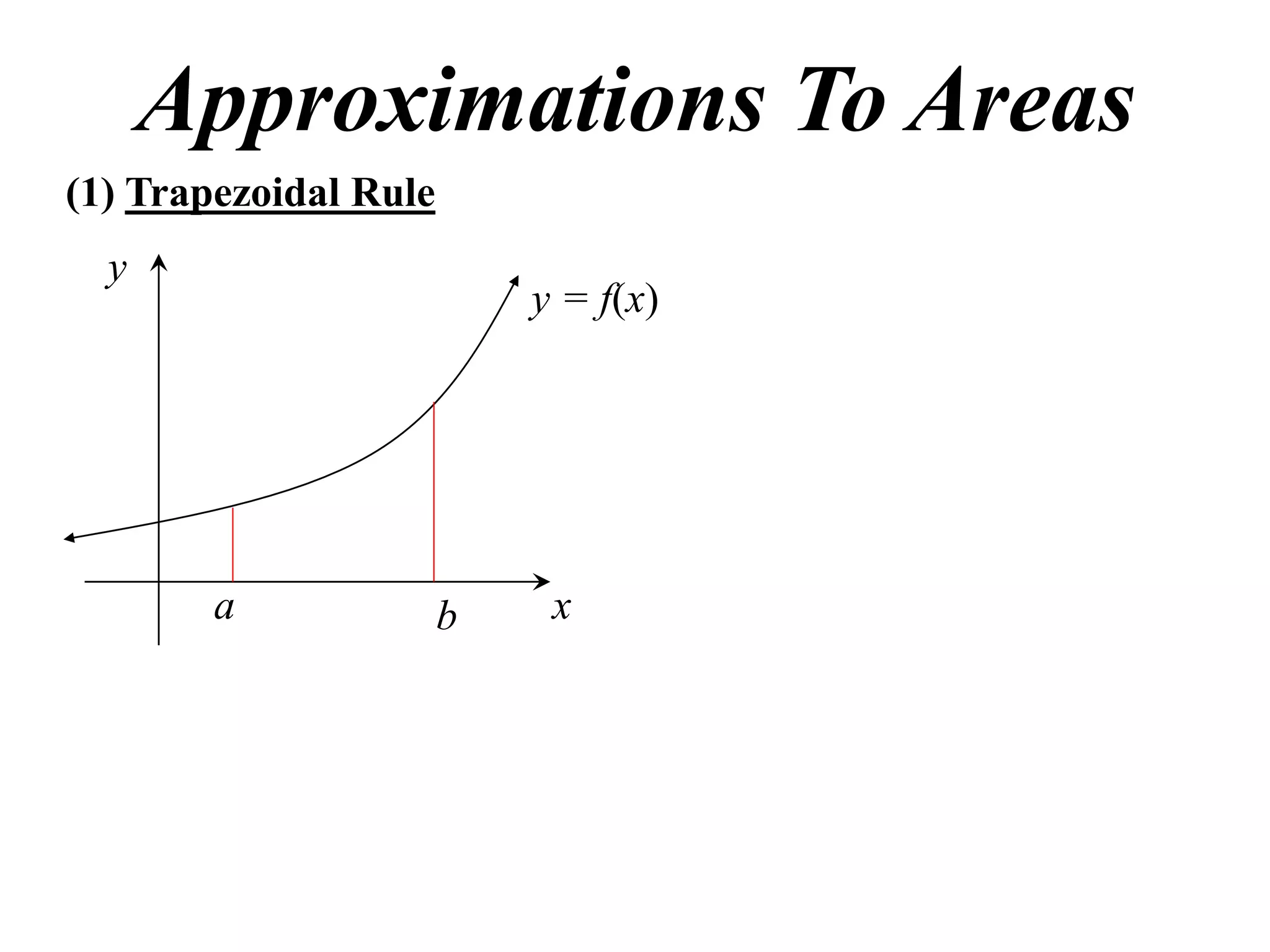
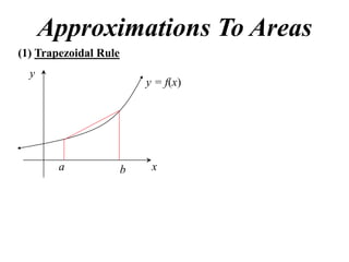
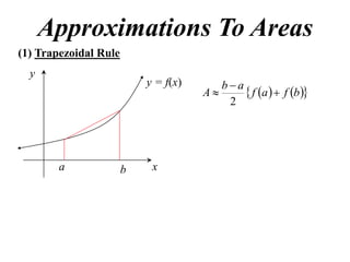
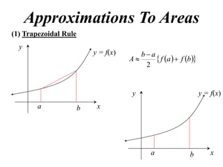
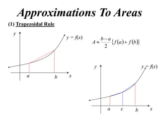
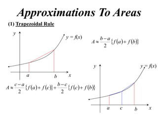
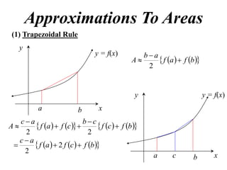
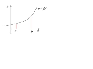
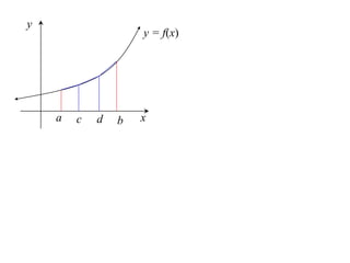
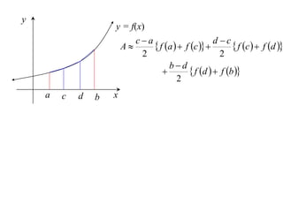
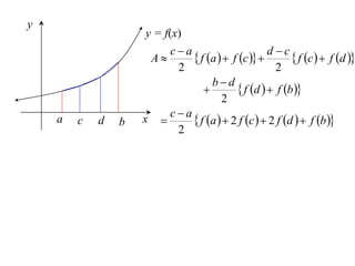
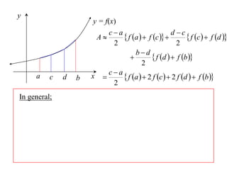
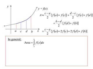
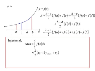
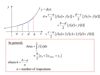
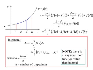
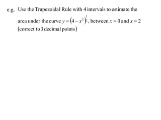
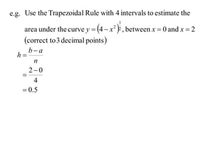
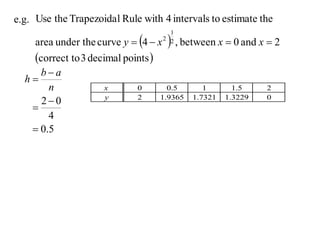
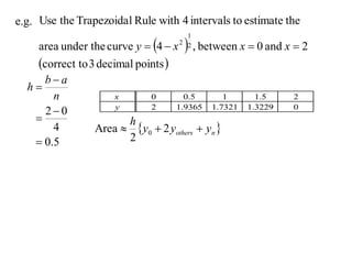
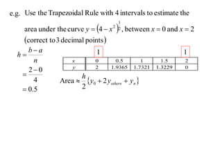
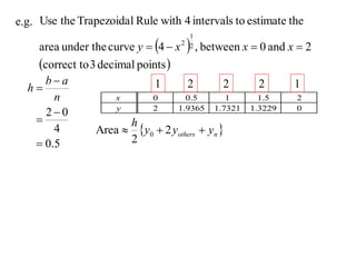
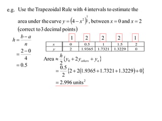
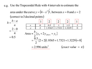
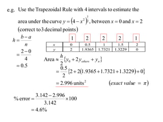
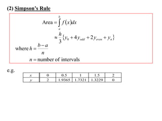
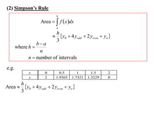
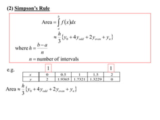
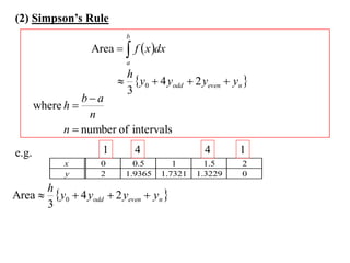
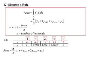
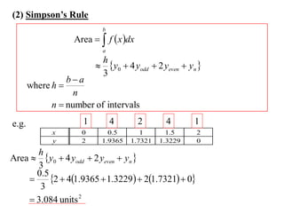
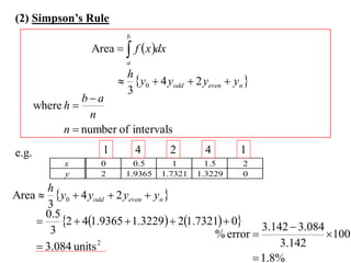
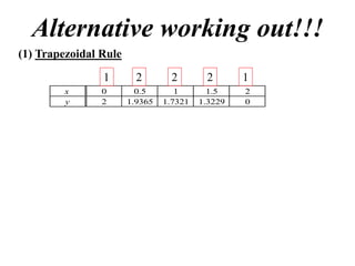
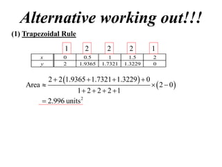
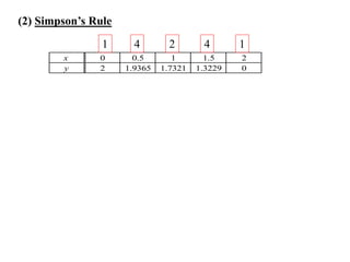
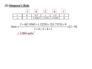
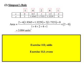
SlideShare a Scribd company logo
Approximations To Areas
(1) Trapezoidal Rule
  y
                           y = f(x)


        a              b    x
Approximations To Areas
(1) Trapezoidal Rule
  y
                           y = f(x)


        a              b    x
Approximations To Areas
(1) Trapezoidal Rule
  y
                           y = f(x)      ba
                                      A      f a   f b 
                                          2


        a              b    x
Approximations To Areas
(1) Trapezoidal Rule
  y
                           y = f(x)      ba
                                      A      f a   f b 
                                          2


                                       y                          y = f(x)
        a              b    x


                                              a             b         x
Approximations To Areas
(1) Trapezoidal Rule
  y
                           y = f(x)      ba
                                      A      f a   f b 
                                          2


                                       y                          y = f(x)
        a              b    x


                                              a     c       b         x
Approximations To Areas
 (1) Trapezoidal Rule
    y
                                 y = f(x)         ba
                                               A      f a   f b 
                                                   2


                                                y                          y = f(x)
           a              b       x
   ca                      bc
A      f a   f c        f c   f b 
    2                        2


                                                       a     c       b         x
Approximations To Areas
 (1) Trapezoidal Rule
    y
                                   y = f(x)          ba
                                                  A      f a   f b 
                                                      2


                                                   y                          y = f(x)
            a               b        x
   ca                      bc
A      f a   f c           f c   f b 
    2                          2
   ca
       f a   2 f c   f b 
    2
                                                          a     c       b         x
y
            y = f(x)


    a   b   x
y
                    y = f(x)


    a   c   d   b   x
y
                    y = f(x)
                           ca                      d c
                        A      f a   f c          f c   f d 
                            2                         2
                                    bd
                                           f d   f b 
                                       2
    a   c   d   b   x
y
                    y = f(x)
                        ca                        d c
                     A        f a   f c           f c   f d 
                          2                          2
                                   bd
                                          f d   f b 
                                      2
    a   c   d   b   x  c  a  f a   2 f c   2 f d   f b 
                          2
y
                      y = f(x)
                          ca                        d c
                       A        f a   f c           f c   f d 
                            2                          2
                                     bd
                                            f d   f b 
                                        2
     a    c   d   b   x  c  a  f a   2 f c   2 f d   f b 
                            2
In general;
y
                            y = f(x)
                                ca                        d c
                             A        f a   f c           f c   f d 
                                  2                          2
                                           bd
                                                  f d   f b 
                                              2
     a    c    d    b       x  c  a  f a   2 f c   2 f d   f b 
                                  2
In general;             b
              Area   f  x dx
                        a
                     h
                     y0  2 yothers  yn 
                     2
y
                              y = f(x)
                                  ca                        d c
                               A        f a   f c           f c   f d 
                                    2                          2
                                             bd
                                                    f d   f b 
                                                2
     a      c    d    b       x  c  a  f a   2 f c   2 f d   f b 
                                    2
In general;               b
                Area   f  x dx
                          a
                       h
                       y0  2 yothers  yn 
                       2
          ba
where h 
            n
      n  number of trapeziums
y
                              y = f(x)
                                  ca                        d c
                               A        f a   f c           f c   f d 
                                    2                          2
                                             bd
                                                    f d   f b 
                                                2
     a      c    d    b       x  c  a  f a   2 f c   2 f d   f b 
                                    2
In general;               b
                Area   f  x dx
                          a
                       h
                       y0  2 yothers  yn         NOTE: there is
                       2
          ba                                         always one more
where h                                              function value
            n
                                                      than interval
      n  number of trapeziums
e.g. Use the Trapezoida l Rule with 4 intervals to estimate the

     area under the curve y  4  x     , between x  0 and x  2
                                         1
                                       2 2


     correct to 3 decimal points 
e.g. Use the Trapezoida l Rule with 4 intervals to estimate the

     area under the curve y  4  x     , between x  0 and x  2
                                         1
                                       2 2


     correct to 3 decimal points 
     ba
  h
       n
     20
   
       4
    0.5
e.g. Use the Trapezoida l Rule with 4 intervals to estimate the

     area under the curve y  4  x     , between x  0 and x  2
                                         1
                                       2 2


     correct to 3 decimal points 
     ba
  h
       n              x        0        0.5       1       1.5    2
     20              y        2      1.9365   1.7321   1.3229   0
                      h
       4         Area  y0  2 yothers  yn 
    0.5               2
e.g. Use the Trapezoida l Rule with 4 intervals to estimate the

     area under the curve y  4  x     , between x  0 and x  2
                                         1
                                       2 2


     correct to 3 decimal points 
     ba                       1                                 1
  h
       n              x        0        0.5       1       1.5    2
     20              y        2      1.9365   1.7321   1.3229   0
                      h
       4         Area  y0  2 yothers  yn 
    0.5               2
e.g. Use the Trapezoida l Rule with 4 intervals to estimate the

     area under the curve y  4  x     , between x  0 and x  2
                                         1
                                       2 2


     correct to 3 decimal points 
     ba                       1        2        2       2       1
  h
       n              x        0        0.5       1       1.5    2
     20              y        2      1.9365   1.7321   1.3229   0
                       h
       4         Area  y0  2 yothers  yn 
    0.5                2
                        0.5
                           2  21.9365  1.7321  1.3229  0
                         2
                       2.996 units 2
e.g. Use the Trapezoida l Rule with 4 intervals to estimate the

     area under the curve y  4  x     , between x  0 and x  2
                                         1
                                       2 2


     correct to 3 decimal points 
     ba                       1        2        2       2       1
  h
       n              x        0        0.5       1       1.5    2
     20              y        2      1.9365   1.7321   1.3229   0
                       h
       4         Area  y0  2 yothers  yn 
    0.5                2
                        0.5
                           2  21.9365  1.7321  1.3229  0
                         2
                       2.996 units 2           exact value  π 
             3.142  2.996
   % error                100
                 3.142
            4.6%
(2) Simpson’s Rule
(2) Simpson’s Rule
                      b
              Area   f  x dx
                      a
(2) Simpson’s Rule
                       b
              Area   f  x dx
                       a
                      h
                      y0  4 yodd  2 yeven  yn 
                      3
(2) Simpson’s Rule
                       b
               Area   f  x dx
                       a
                      h
                      y0  4 yodd  2 yeven  yn 
                      3
             ba
   where h 
               n
         n  number of intervals
(2) Simpson’s Rule
                           b
                   Area   f  x dx
                           a
                          h
                          y0  4 yodd  2 yeven  yn 
                          3
                 ba
       where h 
                   n
             n  number of intervals
e.g.
             x       0       0.5       1       1.5    2
             y       2     1.9365   1.7321   1.3229   0
      h
Area  y0  4 yodd  2 yeven  yn 
      3
(2) Simpson’s Rule
                           b
                   Area   f  x dx
                           a
                          h
                          y0  4 yodd  2 yeven  yn 
                          3
                 ba
       where h 
                   n
             n  number of intervals
e.g.                 1                                1
             x       0       0.5       1       1.5    2
             y       2     1.9365   1.7321   1.3229   0
      h
Area  y0  4 yodd  2 yeven  yn 
      3
(2) Simpson’s Rule
                           b
                   Area   f  x dx
                           a
                          h
                          y0  4 yodd  2 yeven  yn 
                          3
                 ba
       where h 
                   n
             n  number of intervals
e.g.                 1         4              4       1
             x       0       0.5       1       1.5    2
             y       2     1.9365   1.7321   1.3229   0
      h
Area  y0  4 yodd  2 yeven  yn 
      3
(2) Simpson’s Rule
                           b
                   Area   f  x dx
                           a
                          h
                          y0  4 yodd  2 yeven  yn 
                          3
                 ba
       where h 
                   n
             n  number of intervals
e.g.                 1         4        2     4       1
             x       0       0.5       1       1.5    2
             y       2     1.9365   1.7321   1.3229   0
      h
Area  y0  4 yodd  2 yeven  yn 
      3
      0.5
         2  41.9365  1.3229  21.7321  0
       3
     3.084 units 2
(2) Simpson’s Rule
                           b
                   Area   f  x dx
                           a
                          h
                          y0  4 yodd  2 yeven  yn 
                          3
                 ba
       where h 
                   n
             n  number of intervals
e.g.                 1         4        2     4       1
             x       0       0.5       1       1.5    2
             y       2     1.9365   1.7321   1.3229   0
      h
Area  y0  4 yodd  2 yeven  yn 
      3
      0.5
         2  41.9365  1.3229  21.7321  0 3.142  3.084
       3                                   % error              100
     3.084 units 2                                     3.142
                                                    1.8%
Alternative working out!!!
(1) Trapezoidal Rule
Alternative working out!!!
(1) Trapezoidal Rule
                1        2        2       2       1
        x       0        0.5       1       1.5    2
        y       2      1.9365   1.7321   1.3229   0
Alternative working out!!!
(1) Trapezoidal Rule
                  1       2        2       2         1
        x         0       0.5       1       1.5      2
        y         2     1.9365   1.7321   1.3229     0


             2  2 1.9365  1.7321  1.3229   0
    Area                                              2  0
                     1 2  2  2 1
          2.996 units 2
(2) Simpson’s Rule
                1      4        2       4       1
        x      0       0.5       1       1.5    2
        y      2     1.9365   1.7321   1.3229   0
(2) Simpson’s Rule
                   1       4       2       4       1
        x         0       0.5       1       1.5    2
        y         2     1.9365   1.7321   1.3229   0


             2  4 1.9365  1.3229   2 1.7321  0
    Area                                                  2  0
                         1 4  2  4 1
          3.084 units 2


                        Exercise 11I; odds

                        Exercise 11J; evens

More Related Content

What's hot

Chapter 7 solution of equations
Chapter 7 solution of equationsChapter 7 solution of equations
Chapter 7 solution of equations
paufong
 
ลิมิต
ลิมิตลิมิต
ลิมิต
srisuwanthum
 
Exercise #8 notes
Exercise #8 notesExercise #8 notes
Exercise #8 notes
Kelly Scallion
 
Mathematics sample assignment
Mathematics sample assignmentMathematics sample assignment
Mathematics sample assignment
All Assignment Experts
 
Exercise #10 notes
Exercise #10 notesExercise #10 notes
Exercise #10 notes
Kelly Scallion
 
calculo vectorial
calculo vectorialcalculo vectorial
calculo vectorial
Chalio Solano
 
Pc12 sol c03_review
Pc12 sol c03_reviewPc12 sol c03_review
Pc12 sol c03_review
Garden City
 
X2 T04 06 curve sketching - roots of functions
X2 T04 06 curve sketching - roots of functionsX2 T04 06 curve sketching - roots of functions
X2 T04 06 curve sketching - roots of functions
Nigel Simmons
 
Pratikum 1 hardiansyah
Pratikum 1 hardiansyahPratikum 1 hardiansyah
Pratikum 1 hardiansyah
Wirha Sykerz
 
Pratikum 2 urai wira s
Pratikum 2 urai wira sPratikum 2 urai wira s
Pratikum 2 urai wira s
Wirha Sykerz
 
Pc12 sol c04_cp
Pc12 sol c04_cpPc12 sol c04_cp
Pc12 sol c04_cp
Garden City
 
11X1 T14 04 areas
11X1 T14 04 areas11X1 T14 04 areas
11X1 T14 04 areas
Nigel Simmons
 
X2 t07 06 roots of functions (2012)
X2 t07 06 roots of functions (2012)X2 t07 06 roots of functions (2012)
X2 t07 06 roots of functions (2012)
Nigel Simmons
 

What's hot (13)

Chapter 7 solution of equations
Chapter 7 solution of equationsChapter 7 solution of equations
Chapter 7 solution of equations
 
ลิมิต
ลิมิตลิมิต
ลิมิต
 
Exercise #8 notes
Exercise #8 notesExercise #8 notes
Exercise #8 notes
 
Mathematics sample assignment
Mathematics sample assignmentMathematics sample assignment
Mathematics sample assignment
 
Exercise #10 notes
Exercise #10 notesExercise #10 notes
Exercise #10 notes
 
calculo vectorial
calculo vectorialcalculo vectorial
calculo vectorial
 
Pc12 sol c03_review
Pc12 sol c03_reviewPc12 sol c03_review
Pc12 sol c03_review
 
X2 T04 06 curve sketching - roots of functions
X2 T04 06 curve sketching - roots of functionsX2 T04 06 curve sketching - roots of functions
X2 T04 06 curve sketching - roots of functions
 
Pratikum 1 hardiansyah
Pratikum 1 hardiansyahPratikum 1 hardiansyah
Pratikum 1 hardiansyah
 
Pratikum 2 urai wira s
Pratikum 2 urai wira sPratikum 2 urai wira s
Pratikum 2 urai wira s
 
Pc12 sol c04_cp
Pc12 sol c04_cpPc12 sol c04_cp
Pc12 sol c04_cp
 
11X1 T14 04 areas
11X1 T14 04 areas11X1 T14 04 areas
11X1 T14 04 areas
 
X2 t07 06 roots of functions (2012)
X2 t07 06 roots of functions (2012)X2 t07 06 roots of functions (2012)
X2 t07 06 roots of functions (2012)
 

Viewers also liked

X2 T01 10 locus & complex nos 1 (2010)
X2 T01 10 locus & complex nos 1 (2010)X2 T01 10 locus & complex nos 1 (2010)
X2 T01 10 locus & complex nos 1 (2010)Nigel Simmons
 
11 X1 T04 05 sine rule (2010)
11 X1 T04 05 sine rule (2010)11 X1 T04 05 sine rule (2010)
11 X1 T04 05 sine rule (2010)
Nigel Simmons
 
X2 T08 02 inequality techniques (2010)
X2 T08 02 inequality techniques (2010)X2 T08 02 inequality techniques (2010)
X2 T08 02 inequality techniques (2010)Nigel Simmons
 
11X1 T14 02 geometric series (2010)
11X1 T14 02 geometric series (2010)11X1 T14 02 geometric series (2010)
11X1 T14 02 geometric series (2010)
Nigel Simmons
 
12 x1 t08 06 binomial probability (2012)
12 x1 t08 06 binomial probability (2012)12 x1 t08 06 binomial probability (2012)
12 x1 t08 06 binomial probability (2012)
Nigel Simmons
 
11 x1 t14 10 mathematical induction 3 (2013)
11 x1 t14 10 mathematical induction 3 (2013)11 x1 t14 10 mathematical induction 3 (2013)
11 x1 t14 10 mathematical induction 3 (2013)
Nigel Simmons
 
11 x1 t05 02 gradient (2012)
11 x1 t05 02 gradient (2012)11 x1 t05 02 gradient (2012)
11 x1 t05 02 gradient (2012)
Nigel Simmons
 
11X1 T16 04 areas (2011)
11X1 T16 04 areas (2011)11X1 T16 04 areas (2011)
11X1 T16 04 areas (2011)
Nigel Simmons
 
11 x1 t13 06 tangent theorems 2
11 x1 t13 06 tangent theorems 211 x1 t13 06 tangent theorems 2
11 x1 t13 06 tangent theorems 2
Nigel Simmons
 
X2 t06 01 acceleration (2012)
X2 t06 01 acceleration (2012)X2 t06 01 acceleration (2012)
X2 t06 01 acceleration (2012)
Nigel Simmons
 
11 x1 t03 05 regions in the plane (2012)
11 x1 t03 05 regions in the plane (2012)11 x1 t03 05 regions in the plane (2012)
11 x1 t03 05 regions in the plane (2012)
Nigel Simmons
 
11x1 t02 01 real numbers - 2012
11x1 t02 01 real numbers  - 201211x1 t02 01 real numbers  - 2012
11x1 t02 01 real numbers - 2012
Nigel Simmons
 
11 x1 t05 02 permutations ii (2012)
11 x1 t05 02 permutations ii (2012)11 x1 t05 02 permutations ii (2012)
11 x1 t05 02 permutations ii (2012)
Nigel Simmons
 
11 x1 t13 07 products of intercepts (2013)
11 x1 t13 07 products of intercepts (2013)11 x1 t13 07 products of intercepts (2013)
11 x1 t13 07 products of intercepts (2013)
Nigel Simmons
 
11 x1 t13 04 converse theorems (2013)
11 x1 t13 04 converse theorems (2013)11 x1 t13 04 converse theorems (2013)
11 x1 t13 04 converse theorems (2013)
Nigel Simmons
 
11 x1 t04 03 pythagorean trig identities (2012)
11 x1 t04 03 pythagorean trig identities (2012)11 x1 t04 03 pythagorean trig identities (2012)
11 x1 t04 03 pythagorean trig identities (2012)Nigel Simmons
 
11 x1 t12 07 primitive function (2013)
11 x1 t12 07 primitive function (2013)11 x1 t12 07 primitive function (2013)
11 x1 t12 07 primitive function (2013)
Nigel Simmons
 
11 x1 t16 05 volumes (2013)
11 x1 t16 05 volumes (2013)11 x1 t16 05 volumes (2013)
11 x1 t16 05 volumes (2013)
Nigel Simmons
 
11 x1 t16 07 approximations (2013)
11 x1 t16 07 approximations (2013)11 x1 t16 07 approximations (2013)
11 x1 t16 07 approximations (2013)
Nigel Simmons
 
11 x1 t01 09 simultaneous equations (2012)
11 x1 t01 09 simultaneous equations (2012)11 x1 t01 09 simultaneous equations (2012)
11 x1 t01 09 simultaneous equations (2012)
Nigel Simmons
 

Viewers also liked (20)

X2 T01 10 locus & complex nos 1 (2010)
X2 T01 10 locus & complex nos 1 (2010)X2 T01 10 locus & complex nos 1 (2010)
X2 T01 10 locus & complex nos 1 (2010)
 
11 X1 T04 05 sine rule (2010)
11 X1 T04 05 sine rule (2010)11 X1 T04 05 sine rule (2010)
11 X1 T04 05 sine rule (2010)
 
X2 T08 02 inequality techniques (2010)
X2 T08 02 inequality techniques (2010)X2 T08 02 inequality techniques (2010)
X2 T08 02 inequality techniques (2010)
 
11X1 T14 02 geometric series (2010)
11X1 T14 02 geometric series (2010)11X1 T14 02 geometric series (2010)
11X1 T14 02 geometric series (2010)
 
12 x1 t08 06 binomial probability (2012)
12 x1 t08 06 binomial probability (2012)12 x1 t08 06 binomial probability (2012)
12 x1 t08 06 binomial probability (2012)
 
11 x1 t14 10 mathematical induction 3 (2013)
11 x1 t14 10 mathematical induction 3 (2013)11 x1 t14 10 mathematical induction 3 (2013)
11 x1 t14 10 mathematical induction 3 (2013)
 
11 x1 t05 02 gradient (2012)
11 x1 t05 02 gradient (2012)11 x1 t05 02 gradient (2012)
11 x1 t05 02 gradient (2012)
 
11X1 T16 04 areas (2011)
11X1 T16 04 areas (2011)11X1 T16 04 areas (2011)
11X1 T16 04 areas (2011)
 
11 x1 t13 06 tangent theorems 2
11 x1 t13 06 tangent theorems 211 x1 t13 06 tangent theorems 2
11 x1 t13 06 tangent theorems 2
 
X2 t06 01 acceleration (2012)
X2 t06 01 acceleration (2012)X2 t06 01 acceleration (2012)
X2 t06 01 acceleration (2012)
 
11 x1 t03 05 regions in the plane (2012)
11 x1 t03 05 regions in the plane (2012)11 x1 t03 05 regions in the plane (2012)
11 x1 t03 05 regions in the plane (2012)
 
11x1 t02 01 real numbers - 2012
11x1 t02 01 real numbers  - 201211x1 t02 01 real numbers  - 2012
11x1 t02 01 real numbers - 2012
 
11 x1 t05 02 permutations ii (2012)
11 x1 t05 02 permutations ii (2012)11 x1 t05 02 permutations ii (2012)
11 x1 t05 02 permutations ii (2012)
 
11 x1 t13 07 products of intercepts (2013)
11 x1 t13 07 products of intercepts (2013)11 x1 t13 07 products of intercepts (2013)
11 x1 t13 07 products of intercepts (2013)
 
11 x1 t13 04 converse theorems (2013)
11 x1 t13 04 converse theorems (2013)11 x1 t13 04 converse theorems (2013)
11 x1 t13 04 converse theorems (2013)
 
11 x1 t04 03 pythagorean trig identities (2012)
11 x1 t04 03 pythagorean trig identities (2012)11 x1 t04 03 pythagorean trig identities (2012)
11 x1 t04 03 pythagorean trig identities (2012)
 
11 x1 t12 07 primitive function (2013)
11 x1 t12 07 primitive function (2013)11 x1 t12 07 primitive function (2013)
11 x1 t12 07 primitive function (2013)
 
11 x1 t16 05 volumes (2013)
11 x1 t16 05 volumes (2013)11 x1 t16 05 volumes (2013)
11 x1 t16 05 volumes (2013)
 
11 x1 t16 07 approximations (2013)
11 x1 t16 07 approximations (2013)11 x1 t16 07 approximations (2013)
11 x1 t16 07 approximations (2013)
 
11 x1 t01 09 simultaneous equations (2012)
11 x1 t01 09 simultaneous equations (2012)11 x1 t01 09 simultaneous equations (2012)
11 x1 t01 09 simultaneous equations (2012)
 

Similar to 11X1 T17 07 approximations

บทที่ 4 ฟังก์ชัน
บทที่ 4 ฟังก์ชันบทที่ 4 ฟังก์ชัน
บทที่ 4 ฟังก์ชัน
Thipayarat Mocha
 
บทที่ 4 ฟังก์ชัน
บทที่ 4 ฟังก์ชันบทที่ 4 ฟังก์ชัน
บทที่ 4 ฟังก์ชัน
Thipayarat Mocha
 
Equations of Tangents and Normals
Equations of Tangents and NormalsEquations of Tangents and Normals
Equations of Tangents and Normals
coburgmaths
 
ฟังก์ชัน(function)
ฟังก์ชัน(function)ฟังก์ชัน(function)
ฟังก์ชัน(function)
Yodhathai Reesrikom
 
Common derivatives integrals_reduced
Common derivatives integrals_reducedCommon derivatives integrals_reduced
Common derivatives integrals_reduced
Kyro Fitkry
 
Pc12 sol c04_cp
Pc12 sol c04_cpPc12 sol c04_cp
Pc12 sol c04_cp
Garden City
 
Formulario de calculo
Formulario de calculoFormulario de calculo
Formulario de calculo
Henry Romero
 
Calculus cheat sheet_integrals
Calculus cheat sheet_integralsCalculus cheat sheet_integrals
Calculus cheat sheet_integrals
UrbanX4
 
0207 ch 2 day 7
0207 ch 2 day 70207 ch 2 day 7
0207 ch 2 day 7
festivalelmo
 
Pc12 sol c04_4-1
Pc12 sol c04_4-1Pc12 sol c04_4-1
Pc12 sol c04_4-1
Garden City
 
11 x1 t04 06 cosine rule (2013)
11 x1 t04 06 cosine rule (2013)11 x1 t04 06 cosine rule (2013)
11 x1 t04 06 cosine rule (2013)
Nigel Simmons
 
11X1 T04 06 cosine rule (2011)
11X1 T04 06 cosine rule (2011)11X1 T04 06 cosine rule (2011)
11X1 T04 06 cosine rule (2011)
Nigel Simmons
 
11 x1 t04 06 cosine rule (2012)
11 x1 t04 06 cosine rule (2012)11 x1 t04 06 cosine rule (2012)
11 x1 t04 06 cosine rule (2012)
Nigel Simmons
 
11 X1 T04 06 cosine rule (2010)
11 X1 T04 06 cosine rule (2010)11 X1 T04 06 cosine rule (2010)
11 X1 T04 06 cosine rule (2010)
Nigel Simmons
 
Figures
FiguresFigures
Figures
Drradz Maths
 
Figures
FiguresFigures
Figures
Drradz Maths
 
11 x1 t01 08 completing the square (2013)
11 x1 t01 08 completing the square (2013)11 x1 t01 08 completing the square (2013)
11 x1 t01 08 completing the square (2013)
Nigel Simmons
 
Cea0001 ppt project
Cea0001 ppt projectCea0001 ppt project
Cea0001 ppt project
cea0001
 
Key pat1 1-53
Key pat1 1-53Key pat1 1-53
Ma4 set-u-s54
Ma4 set-u-s54Ma4 set-u-s54
Ma4 set-u-s54
Koku Love
 

Similar to 11X1 T17 07 approximations (20)

บทที่ 4 ฟังก์ชัน
บทที่ 4 ฟังก์ชันบทที่ 4 ฟังก์ชัน
บทที่ 4 ฟังก์ชัน
 
บทที่ 4 ฟังก์ชัน
บทที่ 4 ฟังก์ชันบทที่ 4 ฟังก์ชัน
บทที่ 4 ฟังก์ชัน
 
Equations of Tangents and Normals
Equations of Tangents and NormalsEquations of Tangents and Normals
Equations of Tangents and Normals
 
ฟังก์ชัน(function)
ฟังก์ชัน(function)ฟังก์ชัน(function)
ฟังก์ชัน(function)
 
Common derivatives integrals_reduced
Common derivatives integrals_reducedCommon derivatives integrals_reduced
Common derivatives integrals_reduced
 
Pc12 sol c04_cp
Pc12 sol c04_cpPc12 sol c04_cp
Pc12 sol c04_cp
 
Formulario de calculo
Formulario de calculoFormulario de calculo
Formulario de calculo
 
Calculus cheat sheet_integrals
Calculus cheat sheet_integralsCalculus cheat sheet_integrals
Calculus cheat sheet_integrals
 
0207 ch 2 day 7
0207 ch 2 day 70207 ch 2 day 7
0207 ch 2 day 7
 
Pc12 sol c04_4-1
Pc12 sol c04_4-1Pc12 sol c04_4-1
Pc12 sol c04_4-1
 
11 x1 t04 06 cosine rule (2013)
11 x1 t04 06 cosine rule (2013)11 x1 t04 06 cosine rule (2013)
11 x1 t04 06 cosine rule (2013)
 
11X1 T04 06 cosine rule (2011)
11X1 T04 06 cosine rule (2011)11X1 T04 06 cosine rule (2011)
11X1 T04 06 cosine rule (2011)
 
11 x1 t04 06 cosine rule (2012)
11 x1 t04 06 cosine rule (2012)11 x1 t04 06 cosine rule (2012)
11 x1 t04 06 cosine rule (2012)
 
11 X1 T04 06 cosine rule (2010)
11 X1 T04 06 cosine rule (2010)11 X1 T04 06 cosine rule (2010)
11 X1 T04 06 cosine rule (2010)
 
Figures
FiguresFigures
Figures
 
Figures
FiguresFigures
Figures
 
11 x1 t01 08 completing the square (2013)
11 x1 t01 08 completing the square (2013)11 x1 t01 08 completing the square (2013)
11 x1 t01 08 completing the square (2013)
 
Cea0001 ppt project
Cea0001 ppt projectCea0001 ppt project
Cea0001 ppt project
 
Key pat1 1-53
Key pat1 1-53Key pat1 1-53
Key pat1 1-53
 
Ma4 set-u-s54
Ma4 set-u-s54Ma4 set-u-s54
Ma4 set-u-s54
 

More from Nigel Simmons

Goodbye slideshare UPDATE
Goodbye slideshare UPDATEGoodbye slideshare UPDATE
Goodbye slideshare UPDATE
Nigel Simmons
 
Goodbye slideshare
Goodbye slideshareGoodbye slideshare
Goodbye slideshare
Nigel Simmons
 
12 x1 t02 02 integrating exponentials (2014)
12 x1 t02 02 integrating exponentials (2014)12 x1 t02 02 integrating exponentials (2014)
12 x1 t02 02 integrating exponentials (2014)Nigel Simmons
 
11 x1 t01 03 factorising (2014)
11 x1 t01 03 factorising (2014)11 x1 t01 03 factorising (2014)
11 x1 t01 03 factorising (2014)
Nigel Simmons
 
11 x1 t01 02 binomial products (2014)
11 x1 t01 02 binomial products (2014)11 x1 t01 02 binomial products (2014)
11 x1 t01 02 binomial products (2014)Nigel Simmons
 
12 x1 t02 01 differentiating exponentials (2014)
12 x1 t02 01 differentiating exponentials (2014)12 x1 t02 01 differentiating exponentials (2014)
12 x1 t02 01 differentiating exponentials (2014)Nigel Simmons
 
11 x1 t01 01 algebra & indices (2014)
11 x1 t01 01 algebra & indices (2014)11 x1 t01 01 algebra & indices (2014)
11 x1 t01 01 algebra & indices (2014)
Nigel Simmons
 
12 x1 t01 03 integrating derivative on function (2013)
12 x1 t01 03 integrating derivative on function (2013)12 x1 t01 03 integrating derivative on function (2013)
12 x1 t01 03 integrating derivative on function (2013)
Nigel Simmons
 
12 x1 t01 02 differentiating logs (2013)
12 x1 t01 02 differentiating logs (2013)12 x1 t01 02 differentiating logs (2013)
12 x1 t01 02 differentiating logs (2013)Nigel Simmons
 
12 x1 t01 01 log laws (2013)
12 x1 t01 01 log laws (2013)12 x1 t01 01 log laws (2013)
12 x1 t01 01 log laws (2013)
Nigel Simmons
 
X2 t02 04 forming polynomials (2013)
X2 t02 04 forming polynomials (2013)X2 t02 04 forming polynomials (2013)
X2 t02 04 forming polynomials (2013)Nigel Simmons
 
X2 t02 03 roots & coefficients (2013)
X2 t02 03 roots & coefficients (2013)X2 t02 03 roots & coefficients (2013)
X2 t02 03 roots & coefficients (2013)
Nigel Simmons
 
X2 t02 02 multiple roots (2013)
X2 t02 02 multiple roots (2013)X2 t02 02 multiple roots (2013)
X2 t02 02 multiple roots (2013)
Nigel Simmons
 
X2 t02 01 factorising complex expressions (2013)
X2 t02 01 factorising complex expressions (2013)X2 t02 01 factorising complex expressions (2013)
X2 t02 01 factorising complex expressions (2013)
Nigel Simmons
 
11 x1 t16 06 derivative times function (2013)
11 x1 t16 06 derivative times function (2013)11 x1 t16 06 derivative times function (2013)
11 x1 t16 06 derivative times function (2013)Nigel Simmons
 
11 x1 t16 04 areas (2013)
11 x1 t16 04 areas (2013)11 x1 t16 04 areas (2013)
11 x1 t16 04 areas (2013)
Nigel Simmons
 
11 x1 t16 03 indefinite integral (2013)
11 x1 t16 03 indefinite integral (2013)11 x1 t16 03 indefinite integral (2013)
11 x1 t16 03 indefinite integral (2013)Nigel Simmons
 
11 x1 t16 02 definite integral (2013)
11 x1 t16 02 definite integral (2013)11 x1 t16 02 definite integral (2013)
11 x1 t16 02 definite integral (2013)
Nigel Simmons
 
11 x1 t16 01 area under curve (2013)
11 x1 t16 01 area under curve (2013)11 x1 t16 01 area under curve (2013)
11 x1 t16 01 area under curve (2013)
Nigel Simmons
 
X2 t01 11 nth roots of unity (2012)
X2 t01 11 nth roots of unity (2012)X2 t01 11 nth roots of unity (2012)
X2 t01 11 nth roots of unity (2012)
Nigel Simmons
 

More from Nigel Simmons (20)

Goodbye slideshare UPDATE
Goodbye slideshare UPDATEGoodbye slideshare UPDATE
Goodbye slideshare UPDATE
 
Goodbye slideshare
Goodbye slideshareGoodbye slideshare
Goodbye slideshare
 
12 x1 t02 02 integrating exponentials (2014)
12 x1 t02 02 integrating exponentials (2014)12 x1 t02 02 integrating exponentials (2014)
12 x1 t02 02 integrating exponentials (2014)
 
11 x1 t01 03 factorising (2014)
11 x1 t01 03 factorising (2014)11 x1 t01 03 factorising (2014)
11 x1 t01 03 factorising (2014)
 
11 x1 t01 02 binomial products (2014)
11 x1 t01 02 binomial products (2014)11 x1 t01 02 binomial products (2014)
11 x1 t01 02 binomial products (2014)
 
12 x1 t02 01 differentiating exponentials (2014)
12 x1 t02 01 differentiating exponentials (2014)12 x1 t02 01 differentiating exponentials (2014)
12 x1 t02 01 differentiating exponentials (2014)
 
11 x1 t01 01 algebra & indices (2014)
11 x1 t01 01 algebra & indices (2014)11 x1 t01 01 algebra & indices (2014)
11 x1 t01 01 algebra & indices (2014)
 
12 x1 t01 03 integrating derivative on function (2013)
12 x1 t01 03 integrating derivative on function (2013)12 x1 t01 03 integrating derivative on function (2013)
12 x1 t01 03 integrating derivative on function (2013)
 
12 x1 t01 02 differentiating logs (2013)
12 x1 t01 02 differentiating logs (2013)12 x1 t01 02 differentiating logs (2013)
12 x1 t01 02 differentiating logs (2013)
 
12 x1 t01 01 log laws (2013)
12 x1 t01 01 log laws (2013)12 x1 t01 01 log laws (2013)
12 x1 t01 01 log laws (2013)
 
X2 t02 04 forming polynomials (2013)
X2 t02 04 forming polynomials (2013)X2 t02 04 forming polynomials (2013)
X2 t02 04 forming polynomials (2013)
 
X2 t02 03 roots & coefficients (2013)
X2 t02 03 roots & coefficients (2013)X2 t02 03 roots & coefficients (2013)
X2 t02 03 roots & coefficients (2013)
 
X2 t02 02 multiple roots (2013)
X2 t02 02 multiple roots (2013)X2 t02 02 multiple roots (2013)
X2 t02 02 multiple roots (2013)
 
X2 t02 01 factorising complex expressions (2013)
X2 t02 01 factorising complex expressions (2013)X2 t02 01 factorising complex expressions (2013)
X2 t02 01 factorising complex expressions (2013)
 
11 x1 t16 06 derivative times function (2013)
11 x1 t16 06 derivative times function (2013)11 x1 t16 06 derivative times function (2013)
11 x1 t16 06 derivative times function (2013)
 
11 x1 t16 04 areas (2013)
11 x1 t16 04 areas (2013)11 x1 t16 04 areas (2013)
11 x1 t16 04 areas (2013)
 
11 x1 t16 03 indefinite integral (2013)
11 x1 t16 03 indefinite integral (2013)11 x1 t16 03 indefinite integral (2013)
11 x1 t16 03 indefinite integral (2013)
 
11 x1 t16 02 definite integral (2013)
11 x1 t16 02 definite integral (2013)11 x1 t16 02 definite integral (2013)
11 x1 t16 02 definite integral (2013)
 
11 x1 t16 01 area under curve (2013)
11 x1 t16 01 area under curve (2013)11 x1 t16 01 area under curve (2013)
11 x1 t16 01 area under curve (2013)
 
X2 t01 11 nth roots of unity (2012)
X2 t01 11 nth roots of unity (2012)X2 t01 11 nth roots of unity (2012)
X2 t01 11 nth roots of unity (2012)
 

Recently uploaded

ANATOMY AND BIOMECHANICS OF HIP JOINT.pdf
ANATOMY AND BIOMECHANICS OF HIP JOINT.pdfANATOMY AND BIOMECHANICS OF HIP JOINT.pdf
ANATOMY AND BIOMECHANICS OF HIP JOINT.pdf
Priyankaranawat4
 
Pengantar Penggunaan Flutter - Dart programming language1.pptx
Pengantar Penggunaan Flutter - Dart programming language1.pptxPengantar Penggunaan Flutter - Dart programming language1.pptx
Pengantar Penggunaan Flutter - Dart programming language1.pptx
Fajar Baskoro
 
Digital Artefact 1 - Tiny Home Environmental Design
Digital Artefact 1 - Tiny Home Environmental DesignDigital Artefact 1 - Tiny Home Environmental Design
Digital Artefact 1 - Tiny Home Environmental Design
amberjdewit93
 
The simplified electron and muon model, Oscillating Spacetime: The Foundation...
The simplified electron and muon model, Oscillating Spacetime: The Foundation...The simplified electron and muon model, Oscillating Spacetime: The Foundation...
The simplified electron and muon model, Oscillating Spacetime: The Foundation...
RitikBhardwaj56
 
Hindi varnamala | hindi alphabet PPT.pdf
Hindi varnamala | hindi alphabet PPT.pdfHindi varnamala | hindi alphabet PPT.pdf
Hindi varnamala | hindi alphabet PPT.pdf
Dr. Mulla Adam Ali
 
Digital Artifact 1 - 10VCD Environments Unit
Digital Artifact 1 - 10VCD Environments UnitDigital Artifact 1 - 10VCD Environments Unit
Digital Artifact 1 - 10VCD Environments Unit
chanes7
 
বাংলাদেশ অর্থনৈতিক সমীক্ষা (Economic Review) ২০২৪ UJS App.pdf
বাংলাদেশ অর্থনৈতিক সমীক্ষা (Economic Review) ২০২৪ UJS App.pdfবাংলাদেশ অর্থনৈতিক সমীক্ষা (Economic Review) ২০২৪ UJS App.pdf
বাংলাদেশ অর্থনৈতিক সমীক্ষা (Economic Review) ২০২৪ UJS App.pdf
eBook.com.bd (প্রয়োজনীয় বাংলা বই)
 
The History of Stoke Newington Street Names
The History of Stoke Newington Street NamesThe History of Stoke Newington Street Names
The History of Stoke Newington Street Names
History of Stoke Newington
 
A Independência da América Espanhola LAPBOOK.pdf
A Independência da América Espanhola LAPBOOK.pdfA Independência da América Espanhola LAPBOOK.pdf
A Independência da América Espanhola LAPBOOK.pdf
Jean Carlos Nunes Paixão
 
Film vocab for eal 3 students: Australia the movie
Film vocab for eal 3 students: Australia the movieFilm vocab for eal 3 students: Australia the movie
Film vocab for eal 3 students: Australia the movie
Nicholas Montgomery
 
Main Java[All of the Base Concepts}.docx
Main Java[All of the Base Concepts}.docxMain Java[All of the Base Concepts}.docx
Main Java[All of the Base Concepts}.docx
adhitya5119
 
Smart-Money for SMC traders good time and ICT
Smart-Money for SMC traders good time and ICTSmart-Money for SMC traders good time and ICT
Smart-Money for SMC traders good time and ICT
simonomuemu
 
PCOS corelations and management through Ayurveda.
PCOS corelations and management through Ayurveda.PCOS corelations and management through Ayurveda.
PCOS corelations and management through Ayurveda.
Dr. Shivangi Singh Parihar
 
Life upper-Intermediate B2 Workbook for student
Life upper-Intermediate B2 Workbook for studentLife upper-Intermediate B2 Workbook for student
Life upper-Intermediate B2 Workbook for student
NgcHiNguyn25
 
BBR 2024 Summer Sessions Interview Training
BBR  2024 Summer Sessions Interview TrainingBBR  2024 Summer Sessions Interview Training
BBR 2024 Summer Sessions Interview Training
Katrina Pritchard
 
The Diamonds of 2023-2024 in the IGRA collection
The Diamonds of 2023-2024 in the IGRA collectionThe Diamonds of 2023-2024 in the IGRA collection
The Diamonds of 2023-2024 in the IGRA collection
Israel Genealogy Research Association
 
writing about opinions about Australia the movie
writing about opinions about Australia the moviewriting about opinions about Australia the movie
writing about opinions about Australia the movie
Nicholas Montgomery
 
How to Manage Your Lost Opportunities in Odoo 17 CRM
How to Manage Your Lost Opportunities in Odoo 17 CRMHow to Manage Your Lost Opportunities in Odoo 17 CRM
How to Manage Your Lost Opportunities in Odoo 17 CRM
Celine George
 
clinical examination of hip joint (1).pdf
clinical examination of hip joint (1).pdfclinical examination of hip joint (1).pdf
clinical examination of hip joint (1).pdf
Priyankaranawat4
 
How to Setup Warehouse & Location in Odoo 17 Inventory
How to Setup Warehouse & Location in Odoo 17 InventoryHow to Setup Warehouse & Location in Odoo 17 Inventory
How to Setup Warehouse & Location in Odoo 17 Inventory
Celine George
 

Recently uploaded (20)

ANATOMY AND BIOMECHANICS OF HIP JOINT.pdf
ANATOMY AND BIOMECHANICS OF HIP JOINT.pdfANATOMY AND BIOMECHANICS OF HIP JOINT.pdf
ANATOMY AND BIOMECHANICS OF HIP JOINT.pdf
 
Pengantar Penggunaan Flutter - Dart programming language1.pptx
Pengantar Penggunaan Flutter - Dart programming language1.pptxPengantar Penggunaan Flutter - Dart programming language1.pptx
Pengantar Penggunaan Flutter - Dart programming language1.pptx
 
Digital Artefact 1 - Tiny Home Environmental Design
Digital Artefact 1 - Tiny Home Environmental DesignDigital Artefact 1 - Tiny Home Environmental Design
Digital Artefact 1 - Tiny Home Environmental Design
 
The simplified electron and muon model, Oscillating Spacetime: The Foundation...
The simplified electron and muon model, Oscillating Spacetime: The Foundation...The simplified electron and muon model, Oscillating Spacetime: The Foundation...
The simplified electron and muon model, Oscillating Spacetime: The Foundation...
 
Hindi varnamala | hindi alphabet PPT.pdf
Hindi varnamala | hindi alphabet PPT.pdfHindi varnamala | hindi alphabet PPT.pdf
Hindi varnamala | hindi alphabet PPT.pdf
 
Digital Artifact 1 - 10VCD Environments Unit
Digital Artifact 1 - 10VCD Environments UnitDigital Artifact 1 - 10VCD Environments Unit
Digital Artifact 1 - 10VCD Environments Unit
 
বাংলাদেশ অর্থনৈতিক সমীক্ষা (Economic Review) ২০২৪ UJS App.pdf
বাংলাদেশ অর্থনৈতিক সমীক্ষা (Economic Review) ২০২৪ UJS App.pdfবাংলাদেশ অর্থনৈতিক সমীক্ষা (Economic Review) ২০২৪ UJS App.pdf
বাংলাদেশ অর্থনৈতিক সমীক্ষা (Economic Review) ২০২৪ UJS App.pdf
 
The History of Stoke Newington Street Names
The History of Stoke Newington Street NamesThe History of Stoke Newington Street Names
The History of Stoke Newington Street Names
 
A Independência da América Espanhola LAPBOOK.pdf
A Independência da América Espanhola LAPBOOK.pdfA Independência da América Espanhola LAPBOOK.pdf
A Independência da América Espanhola LAPBOOK.pdf
 
Film vocab for eal 3 students: Australia the movie
Film vocab for eal 3 students: Australia the movieFilm vocab for eal 3 students: Australia the movie
Film vocab for eal 3 students: Australia the movie
 
Main Java[All of the Base Concepts}.docx
Main Java[All of the Base Concepts}.docxMain Java[All of the Base Concepts}.docx
Main Java[All of the Base Concepts}.docx
 
Smart-Money for SMC traders good time and ICT
Smart-Money for SMC traders good time and ICTSmart-Money for SMC traders good time and ICT
Smart-Money for SMC traders good time and ICT
 
PCOS corelations and management through Ayurveda.
PCOS corelations and management through Ayurveda.PCOS corelations and management through Ayurveda.
PCOS corelations and management through Ayurveda.
 
Life upper-Intermediate B2 Workbook for student
Life upper-Intermediate B2 Workbook for studentLife upper-Intermediate B2 Workbook for student
Life upper-Intermediate B2 Workbook for student
 
BBR 2024 Summer Sessions Interview Training
BBR  2024 Summer Sessions Interview TrainingBBR  2024 Summer Sessions Interview Training
BBR 2024 Summer Sessions Interview Training
 
The Diamonds of 2023-2024 in the IGRA collection
The Diamonds of 2023-2024 in the IGRA collectionThe Diamonds of 2023-2024 in the IGRA collection
The Diamonds of 2023-2024 in the IGRA collection
 
writing about opinions about Australia the movie
writing about opinions about Australia the moviewriting about opinions about Australia the movie
writing about opinions about Australia the movie
 
How to Manage Your Lost Opportunities in Odoo 17 CRM
How to Manage Your Lost Opportunities in Odoo 17 CRMHow to Manage Your Lost Opportunities in Odoo 17 CRM
How to Manage Your Lost Opportunities in Odoo 17 CRM
 
clinical examination of hip joint (1).pdf
clinical examination of hip joint (1).pdfclinical examination of hip joint (1).pdf
clinical examination of hip joint (1).pdf
 
How to Setup Warehouse & Location in Odoo 17 Inventory
How to Setup Warehouse & Location in Odoo 17 InventoryHow to Setup Warehouse & Location in Odoo 17 Inventory
How to Setup Warehouse & Location in Odoo 17 Inventory
 

11X1 T17 07 approximations

  • 1. Approximations To Areas (1) Trapezoidal Rule y y = f(x) a b x
  • 2. Approximations To Areas (1) Trapezoidal Rule y y = f(x) a b x
  • 3. Approximations To Areas (1) Trapezoidal Rule y y = f(x) ba A  f a   f b  2 a b x
  • 4. Approximations To Areas (1) Trapezoidal Rule y y = f(x) ba A  f a   f b  2 y y = f(x) a b x a b x
  • 5. Approximations To Areas (1) Trapezoidal Rule y y = f(x) ba A  f a   f b  2 y y = f(x) a b x a c b x
  • 6. Approximations To Areas (1) Trapezoidal Rule y y = f(x) ba A  f a   f b  2 y y = f(x) a b x ca bc A  f a   f c    f c   f b  2 2 a c b x
  • 7. Approximations To Areas (1) Trapezoidal Rule y y = f(x) ba A  f a   f b  2 y y = f(x) a b x ca bc A  f a   f c    f c   f b  2 2 ca   f a   2 f c   f b  2 a c b x
  • 8. y y = f(x) a b x
  • 9. y y = f(x) a c d b x
  • 10. y y = f(x) ca d c A  f a   f c    f c   f d  2 2 bd   f d   f b  2 a c d b x
  • 11. y y = f(x) ca d c A  f a   f c    f c   f d  2 2 bd   f d   f b  2 a c d b x  c  a  f a   2 f c   2 f d   f b  2
  • 12. y y = f(x) ca d c A  f a   f c    f c   f d  2 2 bd   f d   f b  2 a c d b x  c  a  f a   2 f c   2 f d   f b  2 In general;
  • 13. y y = f(x) ca d c A  f a   f c    f c   f d  2 2 bd   f d   f b  2 a c d b x  c  a  f a   2 f c   2 f d   f b  2 In general; b Area   f  x dx a
  • 14. y y = f(x) ca d c A  f a   f c    f c   f d  2 2 bd   f d   f b  2 a c d b x  c  a  f a   2 f c   2 f d   f b  2 In general; b Area   f  x dx a h  y0  2 yothers  yn  2
  • 15. y y = f(x) ca d c A  f a   f c    f c   f d  2 2 bd   f d   f b  2 a c d b x  c  a  f a   2 f c   2 f d   f b  2 In general; b Area   f  x dx a h  y0  2 yothers  yn  2 ba where h  n n  number of trapeziums
  • 16. y y = f(x) ca d c A  f a   f c    f c   f d  2 2 bd   f d   f b  2 a c d b x  c  a  f a   2 f c   2 f d   f b  2 In general; b Area   f  x dx a h  y0  2 yothers  yn  NOTE: there is 2 ba always one more where h  function value n than interval n  number of trapeziums
  • 17. e.g. Use the Trapezoida l Rule with 4 intervals to estimate the area under the curve y  4  x  , between x  0 and x  2 1 2 2 correct to 3 decimal points 
  • 18. e.g. Use the Trapezoida l Rule with 4 intervals to estimate the area under the curve y  4  x  , between x  0 and x  2 1 2 2 correct to 3 decimal points  ba h n 20  4  0.5
  • 19. e.g. Use the Trapezoida l Rule with 4 intervals to estimate the area under the curve y  4  x  , between x  0 and x  2 1 2 2 correct to 3 decimal points  ba h n x 0 0.5 1 1.5 2 20 y 2 1.9365 1.7321 1.3229 0  4  0.5
  • 20. e.g. Use the Trapezoida l Rule with 4 intervals to estimate the area under the curve y  4  x  , between x  0 and x  2 1 2 2 correct to 3 decimal points  ba h n x 0 0.5 1 1.5 2 20 y 2 1.9365 1.7321 1.3229 0  h 4 Area  y0  2 yothers  yn   0.5 2
  • 21. e.g. Use the Trapezoida l Rule with 4 intervals to estimate the area under the curve y  4  x  , between x  0 and x  2 1 2 2 correct to 3 decimal points  ba 1 1 h n x 0 0.5 1 1.5 2 20 y 2 1.9365 1.7321 1.3229 0  h 4 Area  y0  2 yothers  yn   0.5 2
  • 22. e.g. Use the Trapezoida l Rule with 4 intervals to estimate the area under the curve y  4  x  , between x  0 and x  2 1 2 2 correct to 3 decimal points  ba 1 2 2 2 1 h n x 0 0.5 1 1.5 2 20 y 2 1.9365 1.7321 1.3229 0  h 4 Area  y0  2 yothers  yn   0.5 2
  • 23. e.g. Use the Trapezoida l Rule with 4 intervals to estimate the area under the curve y  4  x  , between x  0 and x  2 1 2 2 correct to 3 decimal points  ba 1 2 2 2 1 h n x 0 0.5 1 1.5 2 20 y 2 1.9365 1.7321 1.3229 0  h 4 Area  y0  2 yothers  yn   0.5 2 0.5  2  21.9365  1.7321  1.3229  0 2  2.996 units 2
  • 24. e.g. Use the Trapezoida l Rule with 4 intervals to estimate the area under the curve y  4  x  , between x  0 and x  2 1 2 2 correct to 3 decimal points  ba 1 2 2 2 1 h n x 0 0.5 1 1.5 2 20 y 2 1.9365 1.7321 1.3229 0  h 4 Area  y0  2 yothers  yn   0.5 2 0.5  2  21.9365  1.7321  1.3229  0 2  2.996 units 2 exact value  π 
  • 25. e.g. Use the Trapezoida l Rule with 4 intervals to estimate the area under the curve y  4  x  , between x  0 and x  2 1 2 2 correct to 3 decimal points  ba 1 2 2 2 1 h n x 0 0.5 1 1.5 2 20 y 2 1.9365 1.7321 1.3229 0  h 4 Area  y0  2 yothers  yn   0.5 2 0.5  2  21.9365  1.7321  1.3229  0 2  2.996 units 2 exact value  π  3.142  2.996 % error  100 3.142  4.6%
  • 27. (2) Simpson’s Rule b Area   f  x dx a
  • 28. (2) Simpson’s Rule b Area   f  x dx a h  y0  4 yodd  2 yeven  yn  3
  • 29. (2) Simpson’s Rule b Area   f  x dx a h  y0  4 yodd  2 yeven  yn  3 ba where h  n n  number of intervals
  • 30. (2) Simpson’s Rule b Area   f  x dx a h  y0  4 yodd  2 yeven  yn  3 ba where h  n n  number of intervals e.g. x 0 0.5 1 1.5 2 y 2 1.9365 1.7321 1.3229 0
  • 31. (2) Simpson’s Rule b Area   f  x dx a h  y0  4 yodd  2 yeven  yn  3 ba where h  n n  number of intervals e.g. x 0 0.5 1 1.5 2 y 2 1.9365 1.7321 1.3229 0 h Area  y0  4 yodd  2 yeven  yn  3
  • 32. (2) Simpson’s Rule b Area   f  x dx a h  y0  4 yodd  2 yeven  yn  3 ba where h  n n  number of intervals e.g. 1 1 x 0 0.5 1 1.5 2 y 2 1.9365 1.7321 1.3229 0 h Area  y0  4 yodd  2 yeven  yn  3
  • 33. (2) Simpson’s Rule b Area   f  x dx a h  y0  4 yodd  2 yeven  yn  3 ba where h  n n  number of intervals e.g. 1 4 4 1 x 0 0.5 1 1.5 2 y 2 1.9365 1.7321 1.3229 0 h Area  y0  4 yodd  2 yeven  yn  3
  • 34. (2) Simpson’s Rule b Area   f  x dx a h  y0  4 yodd  2 yeven  yn  3 ba where h  n n  number of intervals e.g. 1 4 2 4 1 x 0 0.5 1 1.5 2 y 2 1.9365 1.7321 1.3229 0 h Area  y0  4 yodd  2 yeven  yn  3
  • 35. (2) Simpson’s Rule b Area   f  x dx a h  y0  4 yodd  2 yeven  yn  3 ba where h  n n  number of intervals e.g. 1 4 2 4 1 x 0 0.5 1 1.5 2 y 2 1.9365 1.7321 1.3229 0 h Area  y0  4 yodd  2 yeven  yn  3 0.5  2  41.9365  1.3229  21.7321  0 3  3.084 units 2
  • 36. (2) Simpson’s Rule b Area   f  x dx a h  y0  4 yodd  2 yeven  yn  3 ba where h  n n  number of intervals e.g. 1 4 2 4 1 x 0 0.5 1 1.5 2 y 2 1.9365 1.7321 1.3229 0 h Area  y0  4 yodd  2 yeven  yn  3 0.5  2  41.9365  1.3229  21.7321  0 3.142  3.084 3 % error  100  3.084 units 2 3.142  1.8%
  • 37. Alternative working out!!! (1) Trapezoidal Rule
  • 38. Alternative working out!!! (1) Trapezoidal Rule 1 2 2 2 1 x 0 0.5 1 1.5 2 y 2 1.9365 1.7321 1.3229 0
  • 39. Alternative working out!!! (1) Trapezoidal Rule 1 2 2 2 1 x 0 0.5 1 1.5 2 y 2 1.9365 1.7321 1.3229 0 2  2 1.9365  1.7321  1.3229   0 Area    2  0 1 2  2  2 1  2.996 units 2
  • 40. (2) Simpson’s Rule 1 4 2 4 1 x 0 0.5 1 1.5 2 y 2 1.9365 1.7321 1.3229 0
  • 41. (2) Simpson’s Rule 1 4 2 4 1 x 0 0.5 1 1.5 2 y 2 1.9365 1.7321 1.3229 0 2  4 1.9365  1.3229   2 1.7321  0 Area    2  0 1 4  2  4 1  3.084 units 2
  • 42. (2) Simpson’s Rule 1 4 2 4 1 x 0 0.5 1 1.5 2 y 2 1.9365 1.7321 1.3229 0 2  4 1.9365  1.3229   2 1.7321  0 Area    2  0 1 4  2  4 1  3.084 units 2 Exercise 11I; odds Exercise 11J; evens