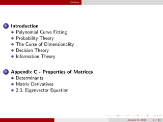
This document provides an outline and introduction to the topics of pattern recognition and machine learning. It begins with an overview of key concepts like probability theory, decision theory, and the curse of dimensionality. It then covers specific techniques like polynomial curve fitting, the Gaussian distribution, and Bayesian curve fitting. The document also includes an appendix on properties of matrices such as determinants, matrix derivatives, and the eigenvector equation.

1. Pattern Recognition and Machine Learning
Eunho Lee
2017-01-03(Tue)
January 8, 2017 1 / 33

2. Outline
1 Introduction
Polynomial Curve Fitting
Probability Theory
The Curse of Dimensionality
Decision Theory
Information Theory
2 Appendix C - Properties of Matrices
Determinants
Matrix Derivatives
2.3. Eigenvector Equation
January 8, 2017 2 / 33

3. Introduction
1. Introduction
Input data set
x ≡ (x1, · · · , xN)T
Target data set
t ≡ (t1, · · · , tN)T
Traning set
Input data set + Target data set
January 8, 2017 3 / 33

4. Introduction
1. Introduction
Data Set
⇓
Probability Theory
⇓
Decision Theory
⇓
Pattern Recognition
* Probability theory provides a
framework for expressing uncentainty
* Decision theory allows us to
exploit the probablistic
representation in order to make
predictions that are optimal
January 8, 2017 4 / 33

5. Introduction Polynomial Curve Fitting
1.1. Polynomial Curve Fitting
y(x, w) = w0 + w1x + w2x2
+ · · · + wMxM
=
M
j=0
wj xj
January 8, 2017 5 / 33

6. Introduction Polynomial Curve Fitting
1.1. Polynomial Curve Fitting
1.1.1. Error Functions
Error Function
E(w) =
1
2
N
n=1
{y(xn, w) − tn}2
(1)
Root-mean-square(RMS) error 1
ERMS = 2E(w∗)/N (2)
* allows us to compare different sizes of data sets
* makes same scale as the target variable
1
w* is a unique solution of the minimization of the error function
January 8, 2017 6 / 33

7. Introduction Polynomial Curve Fitting
1.1. Polynomial Curve Fitting
1.1.2. Over-Fitting
Over-fitting
Very poor representation
January 8, 2017 7 / 33

8. Introduction Polynomial Curve Fitting
1.1. Polynomial Curve Fitting
1.1.3. Modified Error Function
Modified Error Function
E(w) =
1
2
N
n=1
{y(xn, w) − tn}2
+
λ
2
w
2
(3)
prevent the large coefficients w
January 8, 2017 8 / 33

9. Introduction Probability Theory
1.2. Probability Theory
Sum Rule
p(X) =
Y
p(X, Y )
Product Rule
p(X, Y ) = p(Y | X)p(X)
Bayes’ Theorem
p(Y | X) =
p(X | Y )p(Y )
p(X)
January 8, 2017 9 / 33

10. Introduction Probability Theory
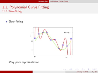
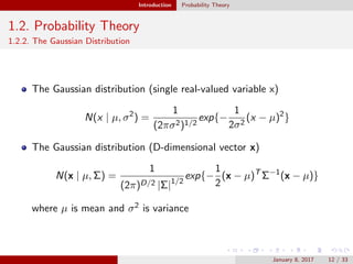
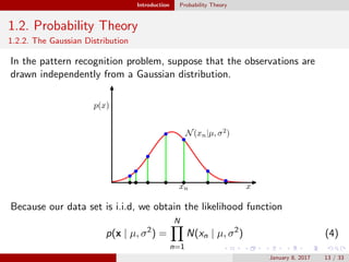
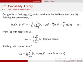
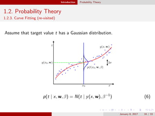
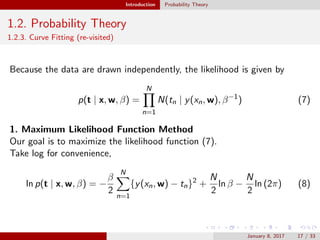
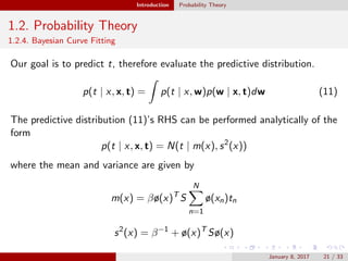
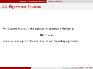
1.2. Probability Theory
Expectation
E[f ] =
x
p(x)f (x)
1
N
N
n=1
f (xn)
Variance
var[f ] = E[(f (x) − E[f (x)])2
]
January 8, 2017 10 / 33

11. Introduction Probability Theory
1.2. Probability Theory
1.2.1. Two Different Probabilities
1. Frequentiest probability (only for large data set)
p(x) =
occurence(x)
N
2. Bayesian probability 2
p(w | D) =
p(D | w)p(w)
p(D)
2
p(wㅣD): posterior, p(w): prior, p(Dㅣw): likelihood function, p(D): evidence
January 8, 2017 11 / 33

12. Introduction Probability Theory
1.2. Probability Theory
1.2.2. The Gaussian Distribution
The Gaussian distribution (single real-valued variable x)
N(x | µ, σ2
) =
1
(2πσ2)1/2
exp{−
1
2σ2
(x − µ)2
}
The Gaussian distribution (D-dimensional vector x)
N(x | µ, Σ) =
1
(2π)D/2 |Σ|1/2
exp{−
1
2
(x − µ)T
Σ−1
(x − µ)}
where µ is mean and σ2 is variance
January 8, 2017 12 / 33

13. Introduction Probability Theory
1.2. Probability Theory
1.2.2. The Gaussian Distribution
In the pattern recognition problem, suppose that the observations are
drawn independently from a Gaussian distribution.
Because our data set is i.i.d, we obtain the likelihood function
p(x | µ, σ2
) =
N
n=1
N(xn | µ, σ2
) (4)
January 8, 2017 13 / 33

14. Introduction Probability Theory
1.2. Probability Theory
1.2.2. The Gaussian Distribution
Our goal is to find µML, σ2
ML which maximize the likelihood function (4).
Take log for convenience,
ln p(x | µ, σ2
) = −
1
2σ2
N
n=1
(xn − µ)2
−
N
2
ln σ2
−
N
2
ln (2π) (5)
From (5) with respect to µ,
µML =
1
N
N
n=1
xn (sample mean)
Similarly, with respect to σ2,
σ2
ML =
1
N
N
n=1
(xn − µML)2
(sample variance)
January 8, 2017 14 / 33

15. Introduction Probability Theory
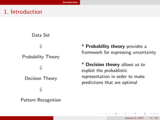
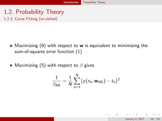
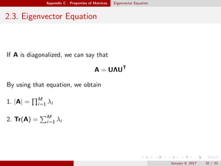
1.2. Probability Theory
1.2.2. The Gaussian Distribution
Therefore,
E[µML] = µ
E[σ2
ML] = (N−1
N )σ2
The figure shows that how variance is biased
January 8, 2017 15 / 33

16. Introduction Probability Theory
1.2. Probability Theory
1.2.3. Curve Fitting (re-visited)
Assume that target value t has a Gaussian distribution.
p(t | x, w, β) = N(t | y(x, w), β−1
) (6)
January 8, 2017 16 / 33

17. Introduction Probability Theory
1.2. Probability Theory
1.2.3. Curve Fitting (re-visited)
Because the data are drawn independently, the likelihood is given by
p(t | x, w, β) =
N
n=1
N(tn | y(xn, w), β−1
) (7)
1. Maximum Likelihood Function Method
Our goal is to maximize the likelihood function (7).
Take log for convenience,
ln p(t | x, w, β) = −
β
2
N
n=1
{y(xn, w) − tn}2
+
N
2
ln β −
N
2
ln (2π) (8)
January 8, 2017 17 / 33

18. Introduction Probability Theory
1.2. Probability Theory
1.2.3. Curve Fitting (re-visited)
Maximizing (8) with respect to w is equivalent to minimizing the
sum-of-squares error function (1)
Maximizing (5) with respect to β gives
1
βML
=
1
N
N
n=1
{y(xn, wML) − tn}2
January 8, 2017 18 / 33

19. Introduction Probability Theory
1.2. Probability Theory
1.2.3. Curve Fitting (re-visited)
2. Maximum Posterior Method (MAP)
Using Bayes’ theorem, the posterior is
p(w | x, t, α, β) ∝ p(t | x, w, β)p(w | α) (9)
Let’s introduce a prior
p(w | α) = N(w | 0, α−1
I) = (
α
2π
)(M+1)/2
exp{−
α
2
wT
w} (10)
Our goal is to maximize the posterior (9)
January 8, 2017 19 / 33

20. Introduction Probability Theory
1.2. Probability Theory
1.2.3. Curve Fitting (re-visited)
Maximizing {posterior} with respect to w
⇔ Maximizing {p(t | x, w, β)p(w | α)} by (9)
⇔ Minimizing {−ln (p(t | x, w, β)p(w | α))}
⇔ Minimizing
β
2
N
n=1{y(xn, w) − tn}2 + α
2 wTw − N
2 ln β + N
2 ln (2π) − ln ( α
2π )(M+1)/2
⇔ Minimizing β
2
N
n=1{y(xn, w) − tn}2 + α
2 wTw
is equivalent to minimizing the modified error function (3) where λ = α
β
January 8, 2017 20 / 33

21. Introduction Probability Theory
1.2. Probability Theory
1.2.4. Bayesian Curve Fitting
Our goal is to predict t, therefore evaluate the predictive distribution.
p(t | x, x, t) = p(t | x, w)p(w | x, t)dw (11)
The predictive distribution (11)’s RHS can be performed analytically of the
form
p(t | x, x, t) = N(t | m(x), s2
(x))
where the mean and variance are given by
m(x) = βø(x)T
S
N
n=1
ø(xn)tn
s2
(x) = β−1
+ ø(x)T
Sø(x)
January 8, 2017 21 / 33

22. Introduction The Curse of Dimensionality
1.3. The Curse of Dimensionality
The severe difficulty that can arise in spaces of many dimensions
How much data do i need to classify?
January 8, 2017 22 / 33

23. Introduction Decision Theory
1.4. Decision Theory
1.4.1. Minimizing the misclassification rate
Rk is decision regions, Ck is k-th class
The boundaries between decision regions are called decision
boundaries
Each decision region need not be contiguous
Classify x to Cm which maximize p(x, Ck)
January 8, 2017 23 / 33

24. Introduction Decision Theory
1.4. Decision Theory
1.4.1. Minimizing the misclassification rate
p(mistake) =
R1
p(x, C2)dx +
R2
p(x, C1)dx
p(x, Ck) = p(Ck | x)p(x)
January 8, 2017 24 / 33

25. Introduction Decision Theory
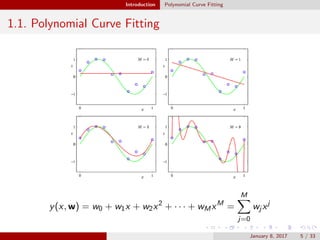
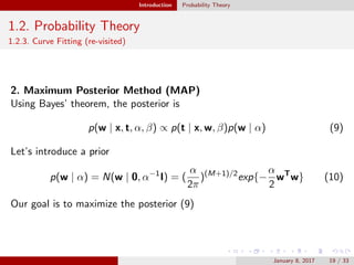
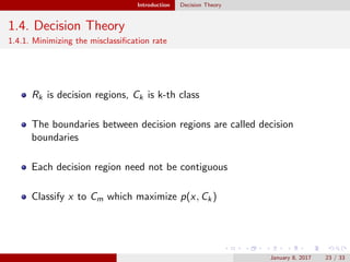
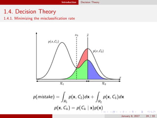
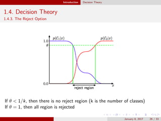
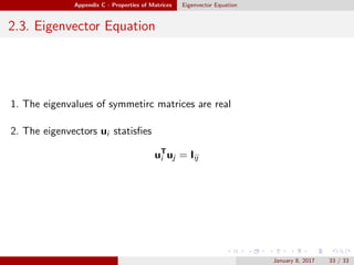
1.4. Decision Theory
1.4.2. Minimizing the expected loss
Dicision’s value is different each other
Minimize the expected loss by using the loss matrix L
E[L] =
k j Rj
Lkj p(x, Ck)dx
January 8, 2017 25 / 33

26. Introduction Decision Theory
1.4. Decision Theory
1.4.3. The Reject Option
If θ < 1/k, then there is no reject region (k is the number of classes)
If θ = 1, then all region is rejected
January 8, 2017 26 / 33

27. Introduction Information Theory
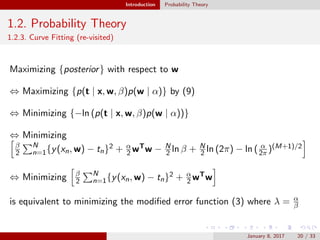
1.5. Infomation Theory
Entropy of the event x (the quantity of information)
h(x) = −log2p(x)
Entropy of the random variable x
H[x] = −
x
p(x)log2p(x)
The distribution that maximizes the differential entropy is the
Gaussian
January 8, 2017 27 / 33

28. Appendix C - Properties of Matrices
2. Appendix C - Properties of Matrices
Determinants
Matrix Derivatives
Eigenvector Equation
January 8, 2017 28 / 33

29. Appendix C - Properties of Matrices Determinants
2.1. Determinants
If A and B are matrices of size N × M, then
IN + ABT
= IM + AT
B
A useful special case is
IN + abT
= 1 + aT
B
where a and b are N-dimensional column vectors
January 8, 2017 29 / 33

30. Appendix C - Properties of Matrices Matrix Derivatives
2.2. Matrix Derivatives
1. ∂
∂x (xTa) = ∂
∂x (aTx) = a
2. ∂
∂x (AB) = ∂A
∂x B + A∂B
∂x
3. ∂
∂x (A−1) = −A−1 ∂A
∂x A−1
4. ∂
∂A Tr(AB) = BT
5. ∂
∂A Tr(A) = I
January 8, 2017 30 / 33

31. Appendix C - Properties of Matrices Eigenvector Equation
2.3. Eigenvector Equation
For a square matrix A, the eigenvector equation is defined by
Aui = λi ui
where ui is an eigenvector and λi is the corresponding eigenvalue
January 8, 2017 31 / 33

32. Appendix C - Properties of Matrices Eigenvector Equation
2.3. Eigenvector Equation
If A is diagonalized, we can say that
A = UΛUT
By using that equation, we obtain
1. |A| = M
i=1 λi
2. Tr(A) = M
i=1 λi
January 8, 2017 32 / 33

33. Appendix C - Properties of Matrices Eigenvector Equation
2.3. Eigenvector Equation
1. The eigenvalues of symmetirc matrices are real
2. The eigenvectors ui statisfies
uT
i uj = Iij
January 8, 2017 33 / 33