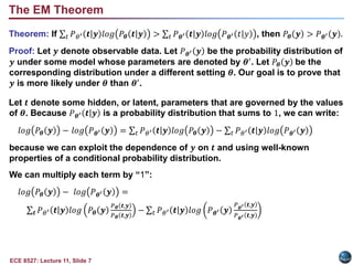
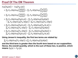
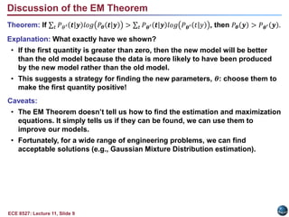
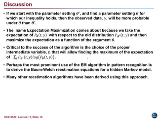
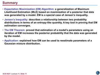
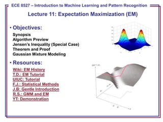
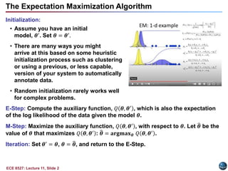
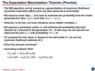
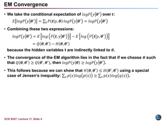
This document discusses the Expectation Maximization (EM) algorithm. EM is an iterative method used to find maximum likelihood estimates of parameters in probabilistic models. It estimates parameters given measurement data, commonly for Gaussian mixture distributions. EM alternates between an expectation (E) step, which computes the expected likelihood including latent variables, and a maximization (M) step, which computes parameter estimates maximizing the expected likelihood. The EM algorithm converges by ensuring that the expected log likelihood is increased with each iteration. Jensen's inequality and the EM theorem prove that this process will converge to a local maximum of the likelihood function.

1. ECE 8443 – Pattern Recognition
ECE 8527 – Introduction to Machine Learning and Pattern Recognition
• Objectives:
Synopsis
Algorithm Preview
Jensen’s Inequality (Special Case)
Theorem and Proof
Gaussian Mixture Modeling
• Resources:
Wiki: EM History
T.D.: EM Tutorial
UIUC: Tutorial
F.J.: Statistical Methods
J.B: Gentle Introduction
R.S.: GMM and EM
YT: Demonstration
Lecture 11: Expectation Maximization (EM)

2. ECE 8527: Lecture 11, Slide 1
• Expectation maximization (EM) is an approach that is used in many ways to
find maximum likelihood estimates of parameters in probabilistic models.
• EM is an iterative optimization method to estimate some unknown parameters
given measurement data. Most commonly used to estimate parameters of a
probabilistic model (e.g., Gaussian mixture distributions).
• Can also be used to discover hidden variables or estimate missing data.
• The intuition behind EM is an old one: alternate between estimating the
unknowns and the hidden variables. This idea has been around for a long
time. However, in 1977, Dempster, et al., proved convergence and explained
the relationship to maximum likelihood estimation.
• EM alternates between performing an expectation (E) step, which computes
an expectation of the likelihood by including the latent variables as if they
were observed, and a maximization (M) step, which computes the maximum
likelihood estimates of the parameters by maximizing the expected likelihood
found on the E step. The parameters found on the M step are then used to
begin another E step, and the process is repeated.
• Cornerstone of important algorithms such as hidden Markov modeling; used
in many fields including human language technology and image processing.
Synopsis

3. ECE 8527: Lecture 11, Slide 2
The Expectation Maximization Algorithm
Initialization:
• Assume you have an initial
model, 𝜽′
. Set 𝜽 = 𝜽′
.
• There are many ways you might
arrive at this based on some heuristic
initialization process such as clustering
or using a previous, or less capable,
version of your system to automatically
annotate data.
• Random initialization rarely works well
for complex problems.
E-Step: Compute the auxiliary function, 𝑄 𝜽, 𝜽′ , which is also the expectation
of the log likelihood of the data given the model 𝜽.
M-Step: Maximize the auxiliary function, 𝑄 𝜽, 𝜽′
, with respect to 𝜽. Let 𝜽 be the
value of 𝜽 that maximizes 𝑄 𝜽, 𝜽′
: 𝜽 = 𝐚𝐫𝐠𝐦𝐚𝐱𝜽 𝑄 𝜽, 𝜽′
.
Iteration: Set 𝜽′ = 𝜽, 𝜽 = 𝜽, and return to the E-Step.

4. ECE 8527: Lecture 11, Slide 3
The Expectation Maximization Theorem (Preview)
• The EM algorithm can be viewed as a generalization of maximum likelihood
parameter estimation (MLE) when the data observed is incomplete.
• We observe some data, 𝑦, and seek to maximize the probability that the model
generated the data, 𝑃𝜽 𝑦 , such that 𝑃𝜽 𝑦 > 𝑃𝜽′ 𝑦 .
• However, to do this, we must introduce some hidden variables, 𝒕.
• We assume a parameter vector, 𝜽, and estimate the probability that each
element of 𝒕 occurred in the generation of 𝑦. In this way, we can assume we
observed the pair 𝒕, 𝑦 with probability 𝑃(𝒕, 𝑦| 𝜽).
• To compute the new value, 𝜽, based on the old model, 𝜽′, we use the
maximum likelihood estimate of 𝜽.
• Does this process converge?
• According to Bayes’ Rule:
𝑃 𝒕, 𝑦|𝜽 = 𝑃 𝒕|𝑦, 𝜽 𝑃 𝑦|𝜽
𝑙𝑜𝑔𝑃 𝑦|𝜽 = 𝑙𝑜𝑔 𝑃 𝒕, 𝑦|𝜽 − 𝑙𝑜𝑔 𝑃 𝒕|𝑦, 𝜽

5. ECE 8527: Lecture 11, Slide 4
EM Convergence
• We take the conditional expectation of 𝑙𝑜𝑔𝑃 𝑦 𝜽′ over 𝒕:
𝐸 𝑙𝑜𝑔𝑃 𝑦 𝜽′
= 𝒕 𝑃 𝒕|𝑦, 𝜽 𝑙𝑜𝑔𝑃 𝑦 𝜽′
= 𝑙𝑜𝑔𝑃 𝑦 𝜽′
• Combining these two expressions:
𝑙𝑜𝑔𝑃 𝑦 𝜽′
= 𝐸 𝑙𝑜𝑔 𝑃 𝒕, 𝑦 𝜽′
− 𝐸 𝑙𝑜𝑔 𝑃 𝒕 𝑦, 𝜽′
= 𝑄 𝜽, 𝜽′
− 𝐻 𝜽, 𝜽′
because the hidden variables t are indirectly linked to 𝜽.
• The convergence of the EM algorithm lies in the fact that if we choose 𝜽 such
that 𝑄 𝜽, 𝜽′ ≥ 𝑄 𝜽′, 𝜽′ , then 𝑙𝑜𝑔𝑃 𝑦|𝜽 ≥ 𝑙𝑜𝑔𝑃 𝑦 𝜽′ .
• This follows because we can show that 𝐻 𝜽, 𝜽′
≤ 𝐻 𝜽′
, 𝜽′
using a special
case of Jensen’s inequality: 𝑥 𝑝 𝑥 𝑙𝑜𝑔 𝑝 𝑥 ≥ 𝑥 𝑝 𝑥 𝑙𝑜𝑔 𝑞 𝑥 .

6. ECE 8527: Lecture 11, Slide 5
Lemma: If 𝑝(𝑥) and 𝑞(𝑥) are two discrete probability distributions, then:
𝑥
𝑝 𝑥 𝑙𝑜𝑔 𝑝 𝑥 ≥
𝑥
𝑝 𝑥 𝑙𝑜𝑔 𝑞 𝑥
with equality if and only if 𝑝(𝑥) = 𝑞(𝑥) for all 𝑥.
Proof:
𝑥
𝑝 𝑥 𝑙𝑜𝑔 𝑝 𝑥 −
𝑥
𝑝 𝑥 𝑙𝑜𝑔 𝑞 𝑥 ≥ 0
𝑥
𝑝 𝑥 𝑙𝑜𝑔 𝑝 𝑥 − 𝑞 𝑥 ≥ 0
𝑥
𝑝 𝑥 𝑙𝑜𝑔
𝑝 𝑥
𝑞 𝑥
≥ 0
𝑥
𝑝 𝑥 𝑙𝑜𝑔
𝑞 𝑥
𝑝 𝑥
≤ 0
𝑥
𝑝 𝑥 𝑙𝑜𝑔
𝑞 𝑥
𝑝 𝑥
≤
𝑥
𝑝 𝑥
𝑞 𝑥
𝑝 𝑥
− 1
The last step follows using a bound for the natural logarithm: 𝑙𝑛 𝑥 ≤ 𝑥 − 1.
.
Special Case of Jensen’s Inequality

7. ECE 8527: Lecture 11, Slide 6
• Continuing in efforts to simplify:
𝑥
𝑝 𝑥 𝑙𝑜𝑔
𝑞 𝑥
𝑝 𝑥
≤
𝑥
𝑝 𝑥
𝑞 𝑥
𝑝 𝑥
− 1 =
𝑥
𝑝 𝑥
𝑞 𝑥
𝑝 𝑥
−
𝑥
𝑝 𝑥
= 𝑥 𝑝 𝑥 − 𝑥 𝑞 𝑥 = 0.
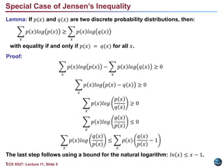
• We note that since both of these functions are probability distributions, they
must sum to 1. Therefore, the inequality holds.
• The general form of Jensen’s inequality relates a convex function of an
integral to the integral of the convex function and is used extensively in
information theory:
If 𝑔(𝑥) is a convex function on 𝑅𝑥, and 𝐸[𝑔(𝑋)] and 𝑔(𝐸[𝑋]) are finite,
then 𝐸[𝑔(𝑋)] ≥ 𝑔(𝐸[𝑋]).
• There are other forms of Jensen’s inequality such as:
 If 𝑝1, 𝑝2, … , 𝑝𝑛 are positive constants that sum to 1 and 𝑓 is a real continuous
function, then:
convex: 𝑓 𝑖=1
𝑛
𝑝𝑖𝑥𝑖 ≤ 𝑖=1
𝑛
𝑝𝑖𝑓 𝑥𝑖 concave: 𝑓 𝑖=1
𝑛
𝑝𝑖𝑥𝑖 ≥ 𝑖=1
𝑛
𝑝𝑖𝑓 𝑥𝑖
Special Case of Jensen’s Inequality

8. ECE 8527: Lecture 11, Slide 7
Theorem: If 𝑡 𝑃𝜃′ 𝒕|𝒚 𝑙𝑜𝑔 𝑃𝜽 𝒕|𝒚 > 𝑡 𝑃𝜽′ 𝒕|𝒚 𝑙𝑜𝑔 𝑃𝜽′ 𝑡|𝑦 , then 𝑃𝜽 𝒚 > 𝑃𝜽′ 𝒚 .
Proof: Let 𝒚 denote observable data. Let 𝑃𝜽′ 𝒚 be the probability distribution of
𝒚 under some model whose parameters are denoted by 𝜽′
. Let 𝑃𝜽 𝒚 be the
corresponding distribution under a different setting 𝜽. Our goal is to prove that
𝒚 is more likely under 𝜽 than 𝜽′.
Let 𝒕 denote some hidden, or latent, parameters that are governed by the values
of 𝜽. Because 𝑃𝜽′ 𝒕|𝒚 is a probability distribution that sums to 1, we can write:
𝑙𝑜𝑔 𝑃𝜽 𝒚 − 𝑙𝑜𝑔 𝑃𝜽′ 𝒚 = 𝑡 𝑃𝜃′ 𝒕|𝒚 𝑙𝑜𝑔 𝑃𝜽 𝒚 − 𝑡 𝑃𝜃′ 𝒕|𝒚 𝑙𝑜𝑔 𝑃𝜽′ 𝒚
because we can exploit the dependence of 𝒚 on 𝒕 and using well-known
properties of a conditional probability distribution.
We can multiply each term by “1”:
𝑙𝑜𝑔 𝑃𝜽 𝒚 − 𝑙𝑜𝑔 𝑃𝜽′ 𝒚 =
𝒕 𝑃𝜃′ 𝒕|𝒚 𝑙𝑜𝑔 𝑃𝜽 𝒚
𝑃𝜽 𝒕,𝒚
𝑃𝜽 𝒕,𝒚
− 𝑡 𝑃𝜃′ 𝒕|𝒚 𝑙𝑜𝑔 𝑃𝜽′ 𝒚
𝑃𝜽′ 𝒕,𝒚
𝑃𝜽′ 𝒕,𝒚
The EM Theorem

9. ECE 8527: Lecture 11, Slide 8
𝑙𝑜𝑔 𝑃𝜽 𝒚 − 𝑙𝑜𝑔 𝑃𝜽′ 𝒚
= 𝒕 𝑃𝜃′ 𝒕|𝒚 𝑙𝑜𝑔
𝑃𝜽 𝒕,𝒚
𝑃𝜽 |
𝒕 𝒚
− 𝑡 𝑃𝜃′ 𝒕|𝒚 𝑙𝑜𝑔
𝑃𝜽′ 𝒕,𝒚
𝑃𝜽′ |
𝒕 𝒚
= 𝒕 𝑃𝜃′ 𝒕|𝒚 𝑙𝑜𝑔
𝑃𝜽 𝒕,𝒚
𝑃𝜽 |
𝒕 𝒚
− 𝑡 𝑃𝜃′ 𝒕|𝒚 𝑙𝑜𝑔
𝑃𝜽′ 𝒕,𝒚
𝑃𝜽′ |
𝒕 𝒚
= 𝒕 𝑃𝜃′ 𝒕|𝒚 𝑙𝑜𝑔 𝑃𝜽 𝒕, 𝒚 − 𝑡 𝑃𝜃′ 𝒕|𝒚 𝑙𝑜𝑔 𝑃𝜽 |
𝒕 𝒚
− 𝑡 𝑃𝜃′ 𝒕|𝒚 𝑙𝑜𝑔 𝑃𝜃′ |
𝒕 𝒚 + 𝒕 𝑃𝜃′ 𝒕|𝒚 𝑙𝑜𝑔 𝑃𝜃′ |
𝒕 𝒚
= 𝒕 𝑃𝜃′ 𝒕|𝒚 𝑙𝑜𝑔 𝑃𝜽 𝒕, 𝒚 − 𝑡 𝑃𝜃′ 𝒕|𝒚 𝑙𝑜𝑔 𝑃𝜽′ 𝒕, 𝒚 +
𝒕 𝑃𝜃′ 𝒕|𝒚 𝑙𝑜𝑔 𝑃𝜃′ |
𝒕 𝒚 − 𝑡 𝑃𝜃′ 𝒕|𝒚 𝑙𝑜𝑔 𝑃𝜽 |
𝒕 𝒚
= 𝒕 𝑃𝜃′ 𝒕|𝒚 𝑙𝑜𝑔 𝑃𝜃′ |
𝒕 𝒚 − 𝑡 𝑃𝜃′ 𝒕|𝒚 𝑙𝑜𝑔 𝑃𝜽 |
𝒕 𝒚 +
𝒕 𝑃𝜃′ 𝒕|𝒚 𝑙𝑜𝑔 𝑃𝜽 𝒕, 𝒚 − 𝑡 𝑃𝜃′ 𝒕|𝒚 𝑙𝑜𝑔 𝑃𝜽′ 𝒕, 𝒚
Using Jensen’s inequality, the first two terms are related by:
𝒕 𝑃𝜃′ 𝒕|𝒚 𝑙𝑜𝑔 𝑃𝜃′ |
𝒕 𝒚 ≥ 𝑡 𝑃𝜃′ 𝒕|𝒚 𝑙𝑜𝑔 𝑃𝜽 |
𝒕 𝒚
and the third term is greater then the fourth term based on our supposition.
Hence, the overall quantity, which is the sum of these two, is positive, which
means 𝑃𝜽 𝒚 > 𝑃𝜽′ 𝒚 .
Proof Of The EM Theorem

10. ECE 8527: Lecture 11, Slide 9
Discussion of the EM Theorem
Theorem: If 𝑡 𝑃𝜃′ 𝒕|𝒚 𝑙𝑜𝑔 𝑃𝜽 𝒕|𝒚 > 𝑡 𝑃𝜽′ 𝒕|𝒚 𝑙𝑜𝑔 𝑃𝜽′ 𝑡|𝑦 , then 𝑃𝜽 𝒚 > 𝑃𝜽′ 𝒚 .
Explanation: What exactly have we shown?
• If the first quantity is greater than zero, then the new model will be better
than the old model because the data is more likely to have been produced
by the new model rather than the old model.
• This suggests a strategy for finding the new parameters, 𝜽: choose them to
make the first quantity positive!
Caveats:
• The EM Theorem doesn’t tell us how to find the estimation and maximization
equations. It simply tells us if they can be found, we can use them to
improve our models.
• Fortunately, for a wide range of engineering problems, we can find
acceptable solutions (e.g., Gaussian Mixture Distribution estimation).

11. ECE 8527: Lecture 11, Slide 10
Discussion
• If we start with the parameter setting 𝜽′, and find a parameter setting 𝜽 for
which our inequality holds, then the observed data, 𝒚, will be more probable
under 𝜽 than 𝜽′
.
• The name Expectation Maximization comes about because we take the
expectation of 𝑃𝜽 𝑡, 𝑦 with respect to the old distribution 𝑃𝜽′ 𝑡, 𝑦 and then
maximize the expectation as a function of the argument 𝜽.
• Critical to the success of the algorithm is the choice of the proper
intermediate variable, t, that will allow finding the maximum of the expectation
of 𝒕 𝑃𝜽′ 𝑡, 𝑦 𝑙𝑜𝑔 𝑃𝜽 𝑡, 𝑦 . .
• Perhaps the most prominent use of the EM algorithm in pattern recognition is
to derive the Baum-Welch reestimation equations for a hidden Markov model.
• Many other reestimation algorithms have been derived using this approach.

12. ECE 8527: Lecture 11, Slide 11
Summary
• Expectation Maximization (EM) Algorithm: a generalization of Maximum
Likelihood Estimation (MLE) based on maximization of a posterior that data
was generated by a model. EM is a special case of Jensen’s inequality.
• Jensen’s Inequality: describes a relationship between two probability
distributions in terms of an entropy-like quantity. A key tool in proving that EM
estimation converges.
• The EM Theorem: proved that estimation of a model’s parameters using an
iteration of EM increases the posterior probability that the data was generated
by the model.
• Application: explained how EM can be used to reestimate parameters of a
Gaussian mixture distribution.

13. ECE 8527: Lecture 11, Slide 12
Example: Estimating Missing Data

14. ECE 8527: Lecture 11, Slide 13
Example: Estimating Missing Data

15. ECE 8527: Lecture 11, Slide 14
Example: Estimating Missing Data

16. ECE 8527: Lecture 11, Slide 15
Example: Estimating Missing Data

17. ECE 8527: Lecture 11, Slide 16
Example: Estimating Missing Data

18. ECE 8527: Lecture 11, Slide 17
Example: Gaussian Mixtures
• An excellent tutorial on Gaussian mixture estimation can be found at
J. Bilmes, EM Estimation
• An interactive demo showing convergence of the estimate can be found at
I. Dinov, Demonstration