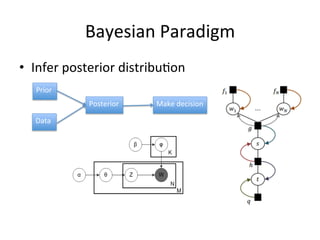
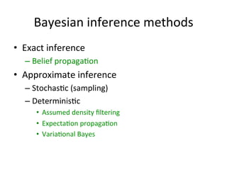
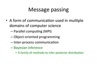
Download as PDF, PPTX


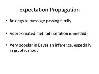


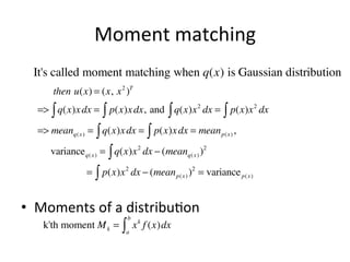
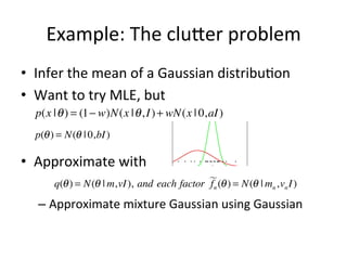
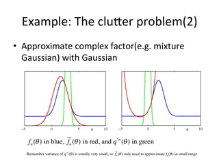
![Distribu(on
Approxima(on
Approximate p(x) with q(x), which belongs to exponential family
Such that: q(x) = h(x)g(η )exp{η T u(x)}
KL( p || q) = − ∫ p(x)In
q(x)
dx = − ∫ p(x)Inq(x)dx + ∫ p(x)Inp(x)dx
p(x)
= − ∫ p(x)Ing(η )dx − ∫ p(x)η T u(x) dx + const
= − Ing(η ) − η T Ε p( x ) [u(x)] + const
where const terms are independent of the natural parameter η
Minimize KL( p || q) by setting the gradient with repect to η to zero:
=> −∇Ing(η ) = Ε p( x ) [u(x)]
By leveraging formula (2.226) in PRML:
=> E q( x ) [u(x)] = −∇Ing(η ) = Ε p( x ) [u(x)]](https://image.slidesharecdn.com/expectationpropagationresearchworkshop-131215193620-phpapp02/85/Expectation-propagation-23-320.jpg)
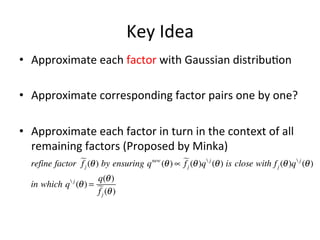
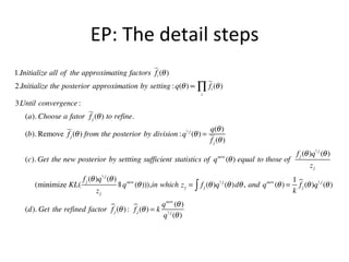
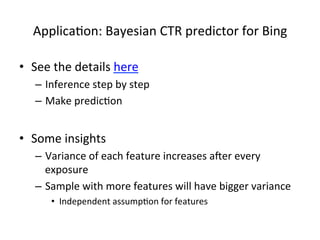
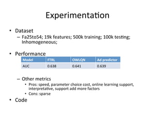
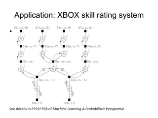

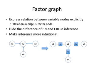
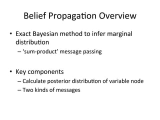
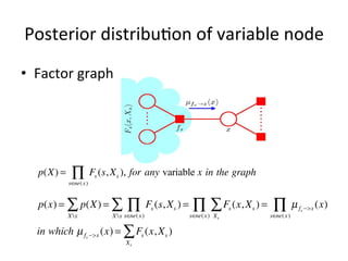
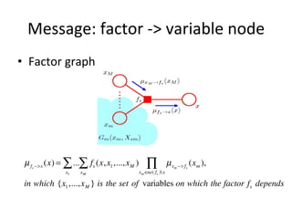
The document discusses the Expectation Propagation (EP) theory and its applications in Bayesian inference, particularly in graphical models and machine learning. It outlines key components of EP, including message passing, factor graphs, and the relationship between variable nodes, and illustrates the method with examples and applications, such as Bayesian click-through rate prediction for Microsoft's Bing. References include essential literature on machine learning and Bayesian methods, including frameworks for Bayesian inference.