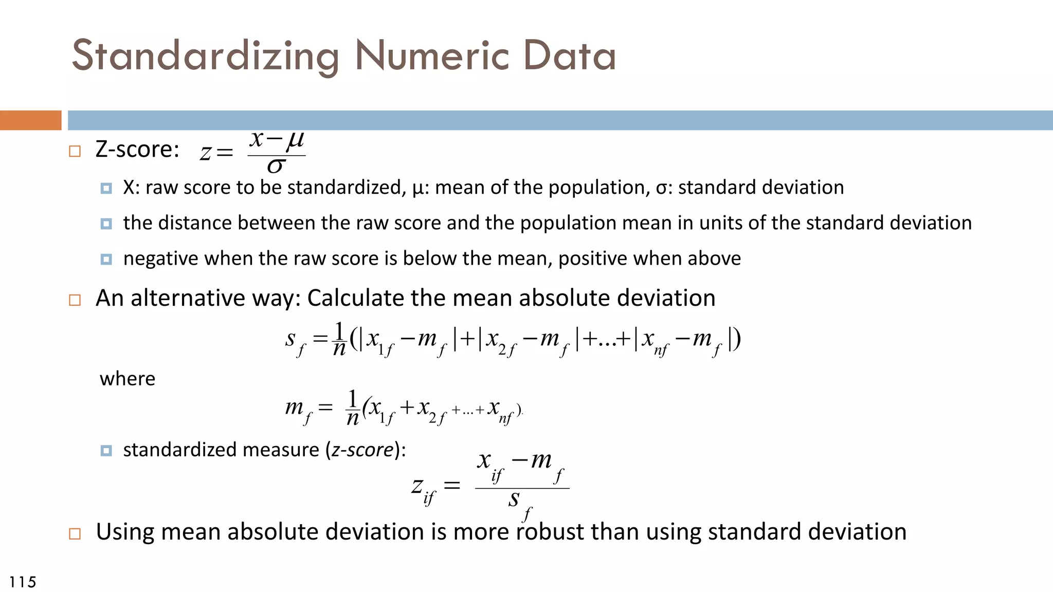
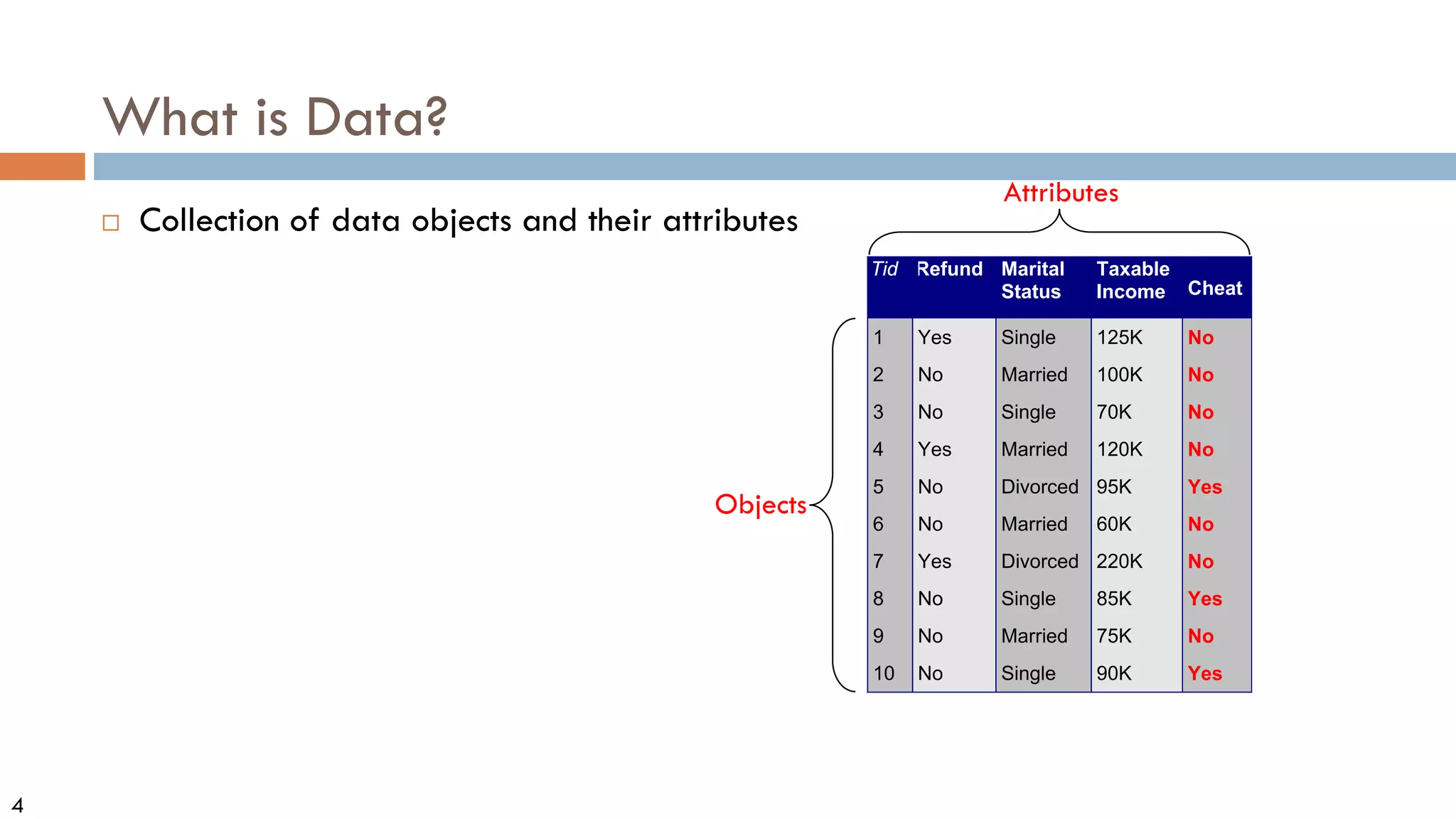
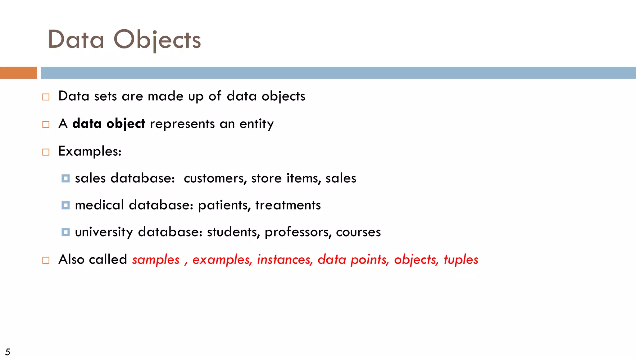
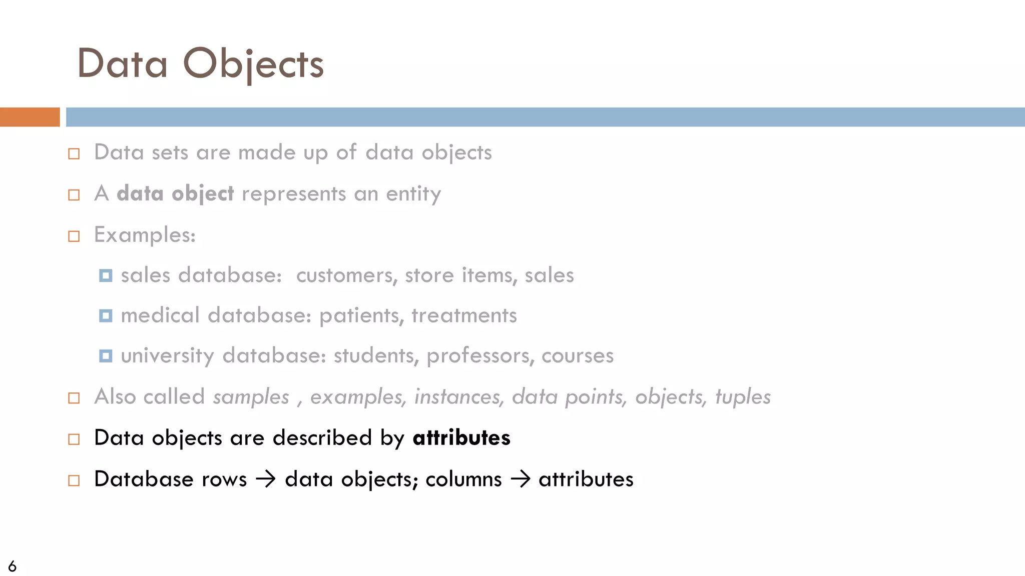
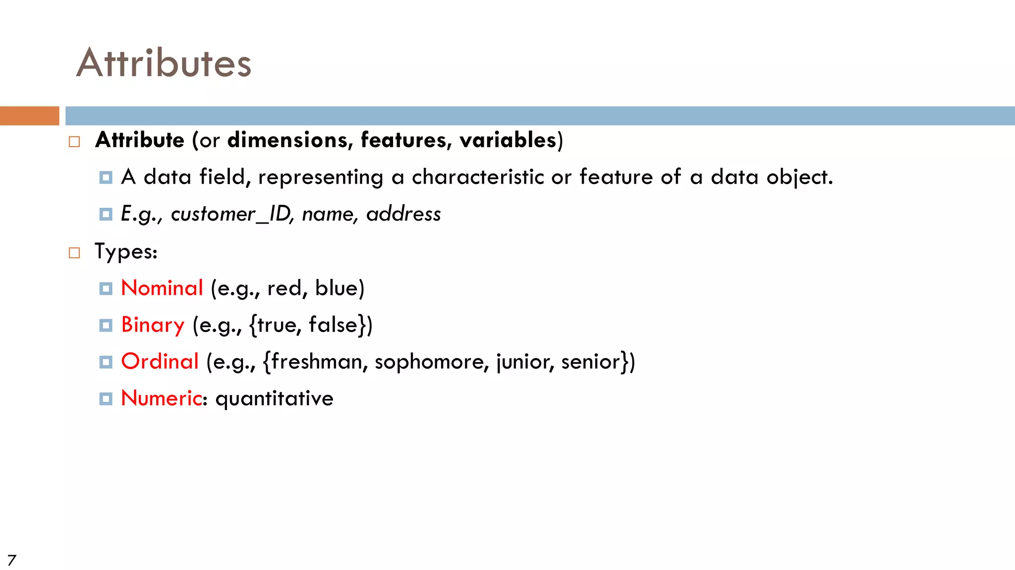
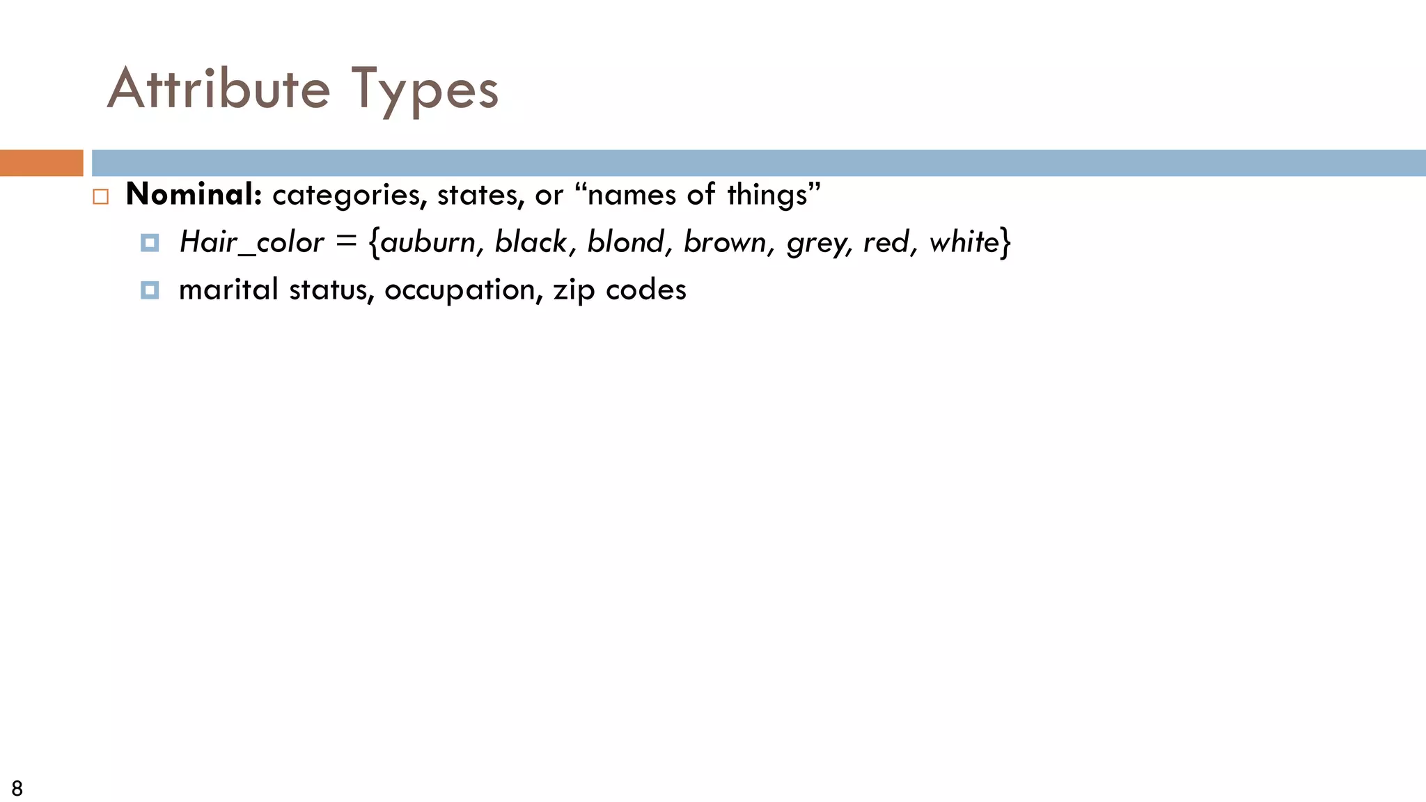
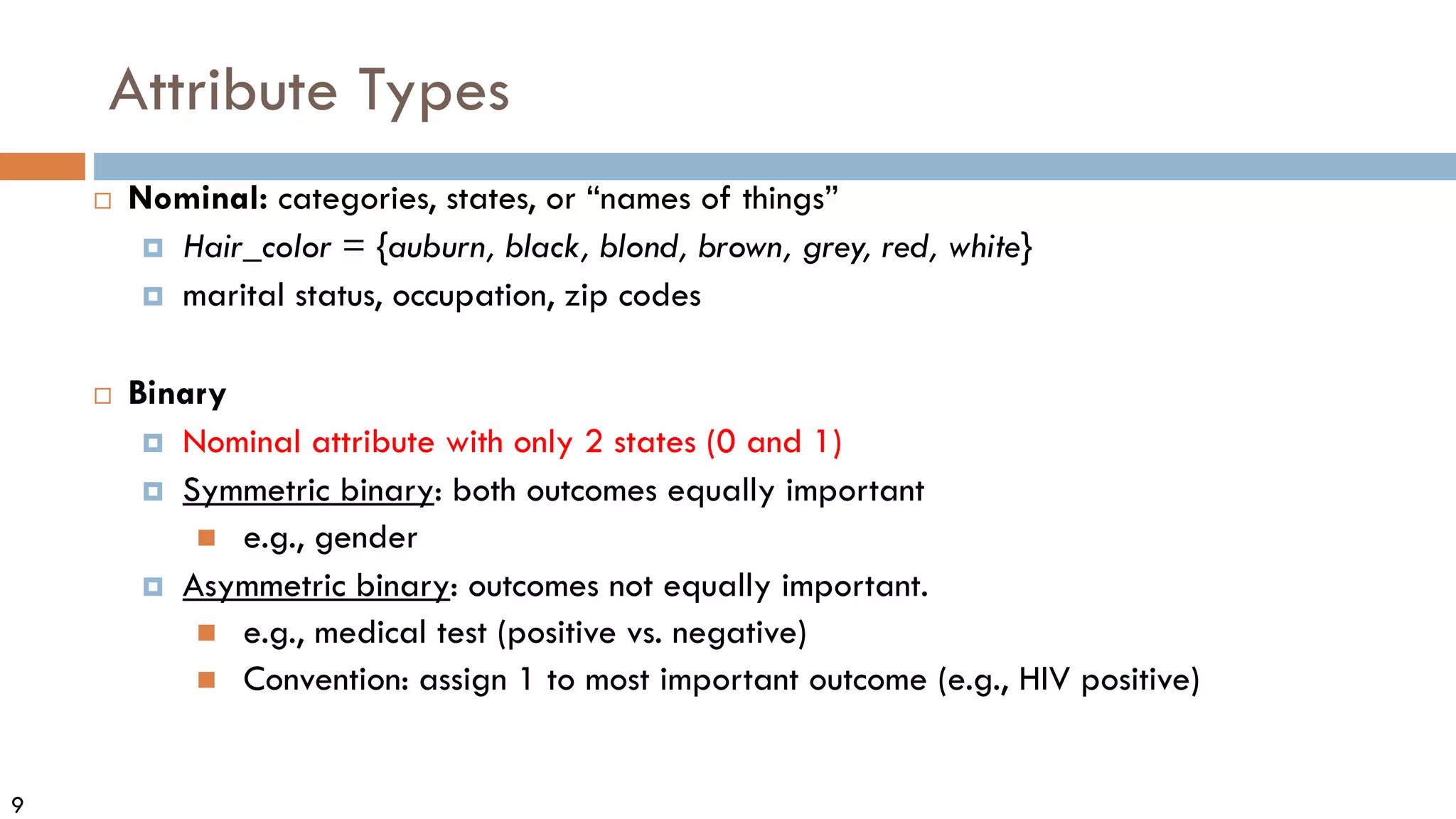
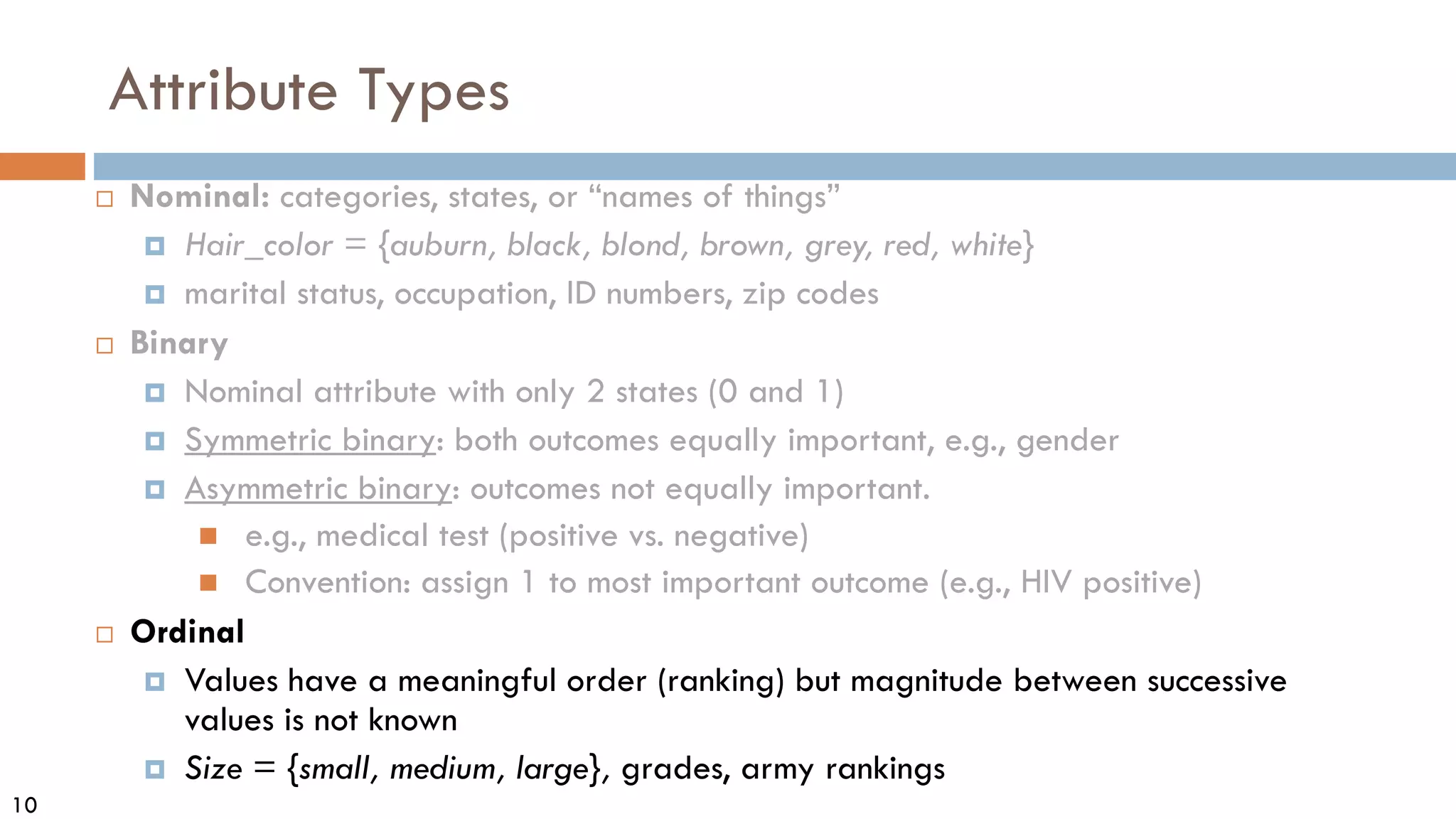
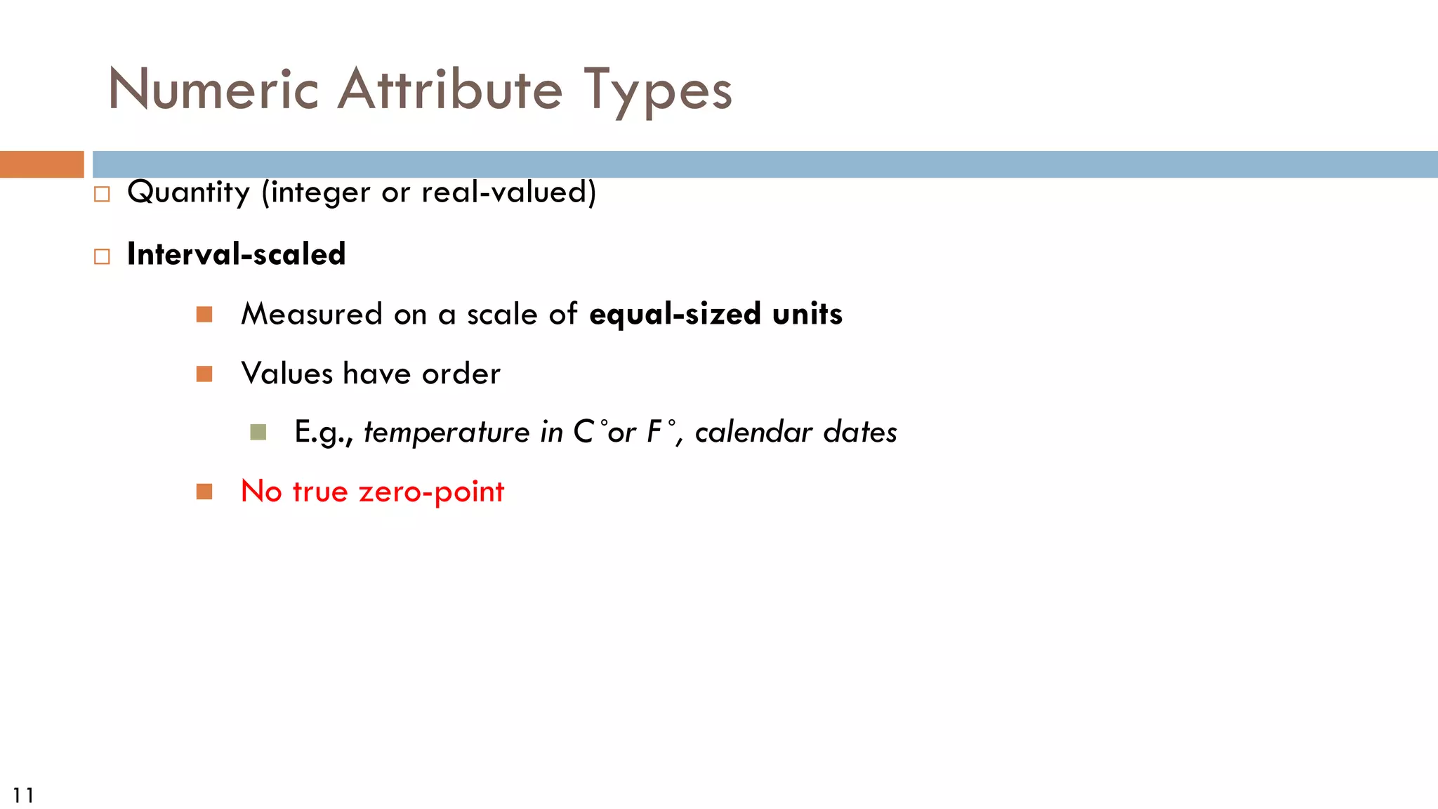
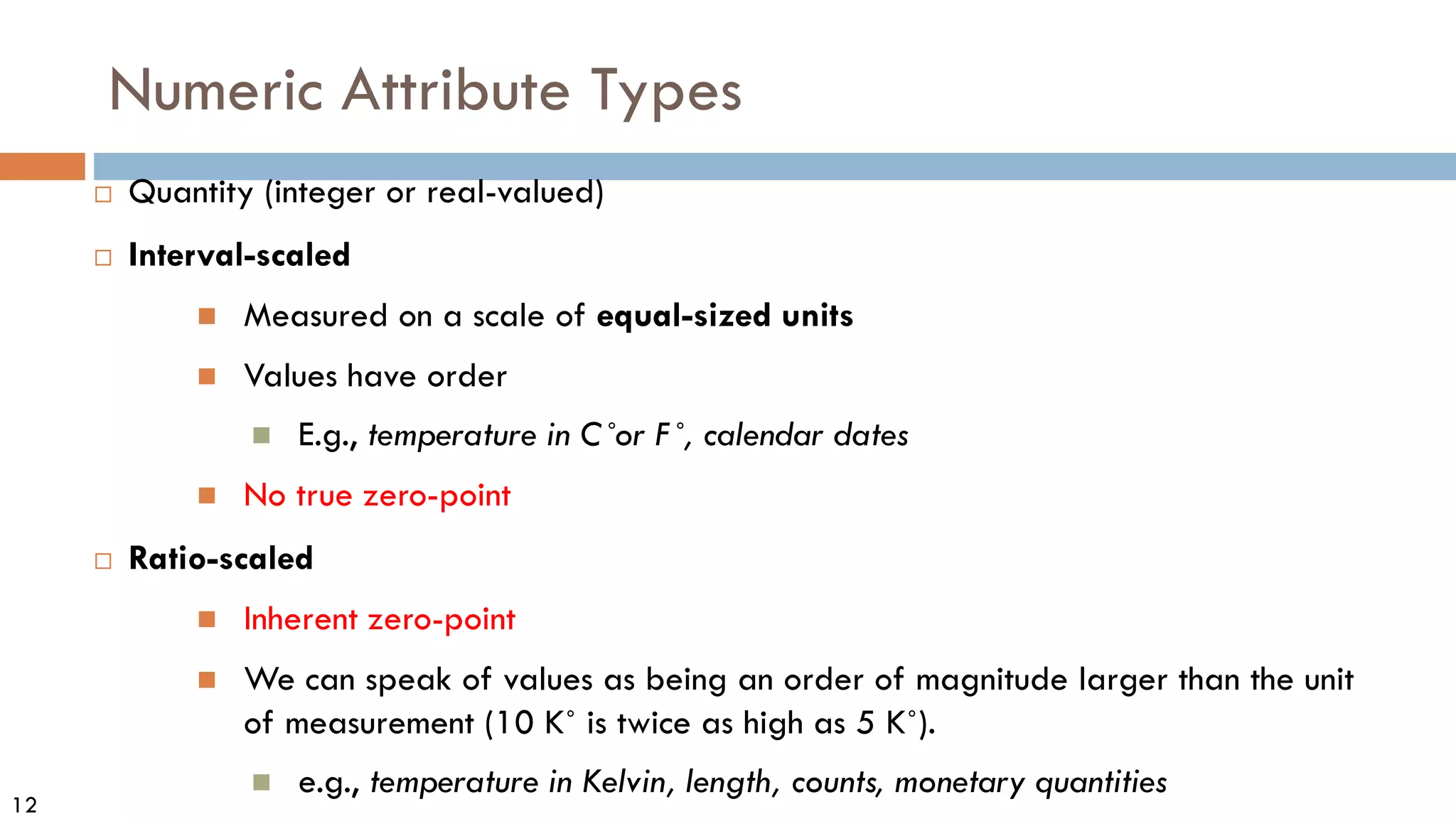
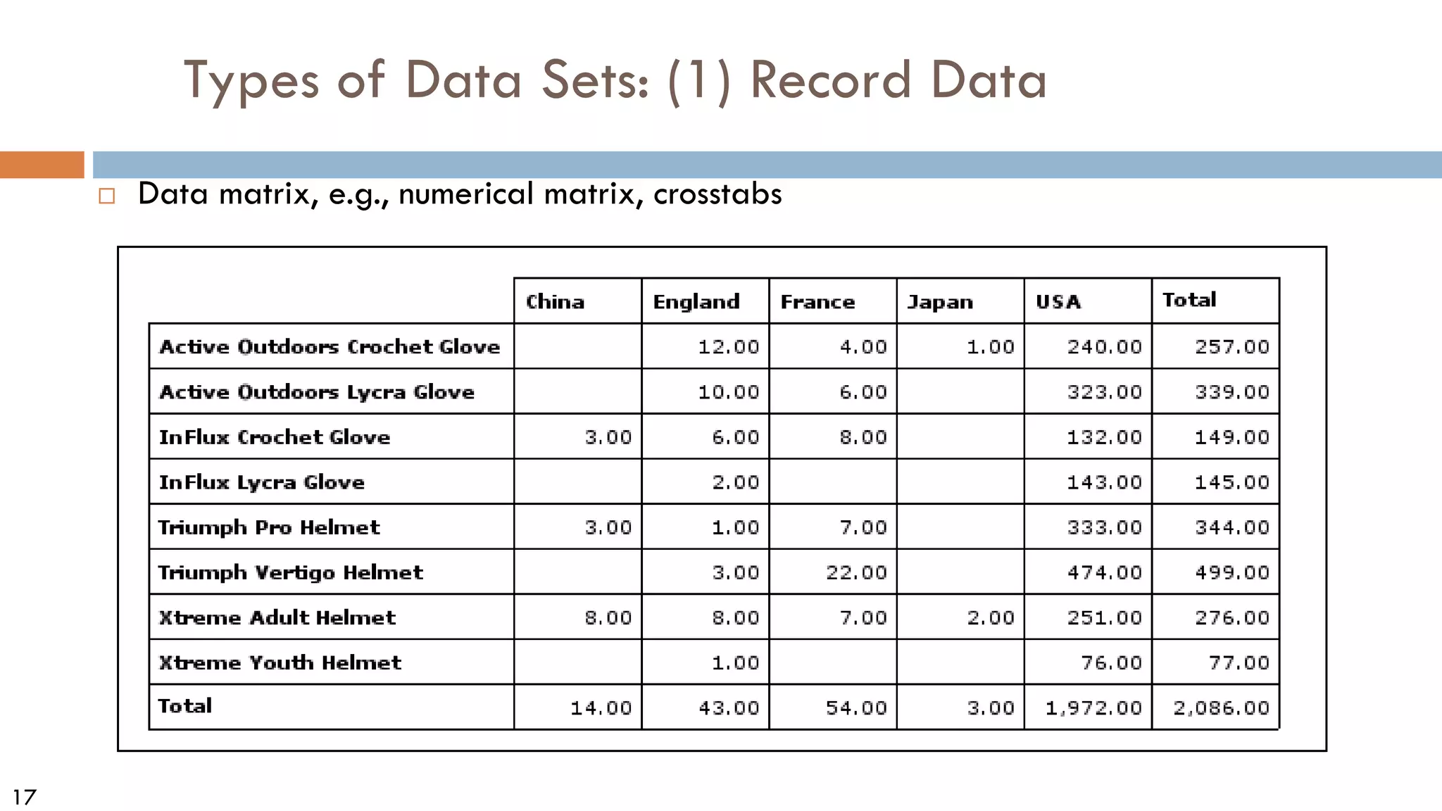
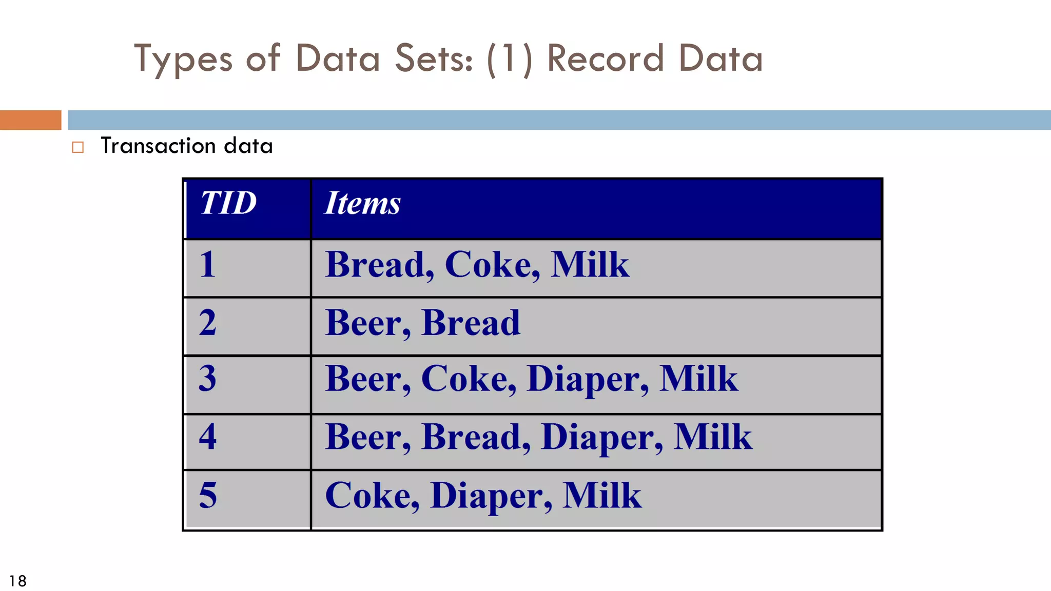
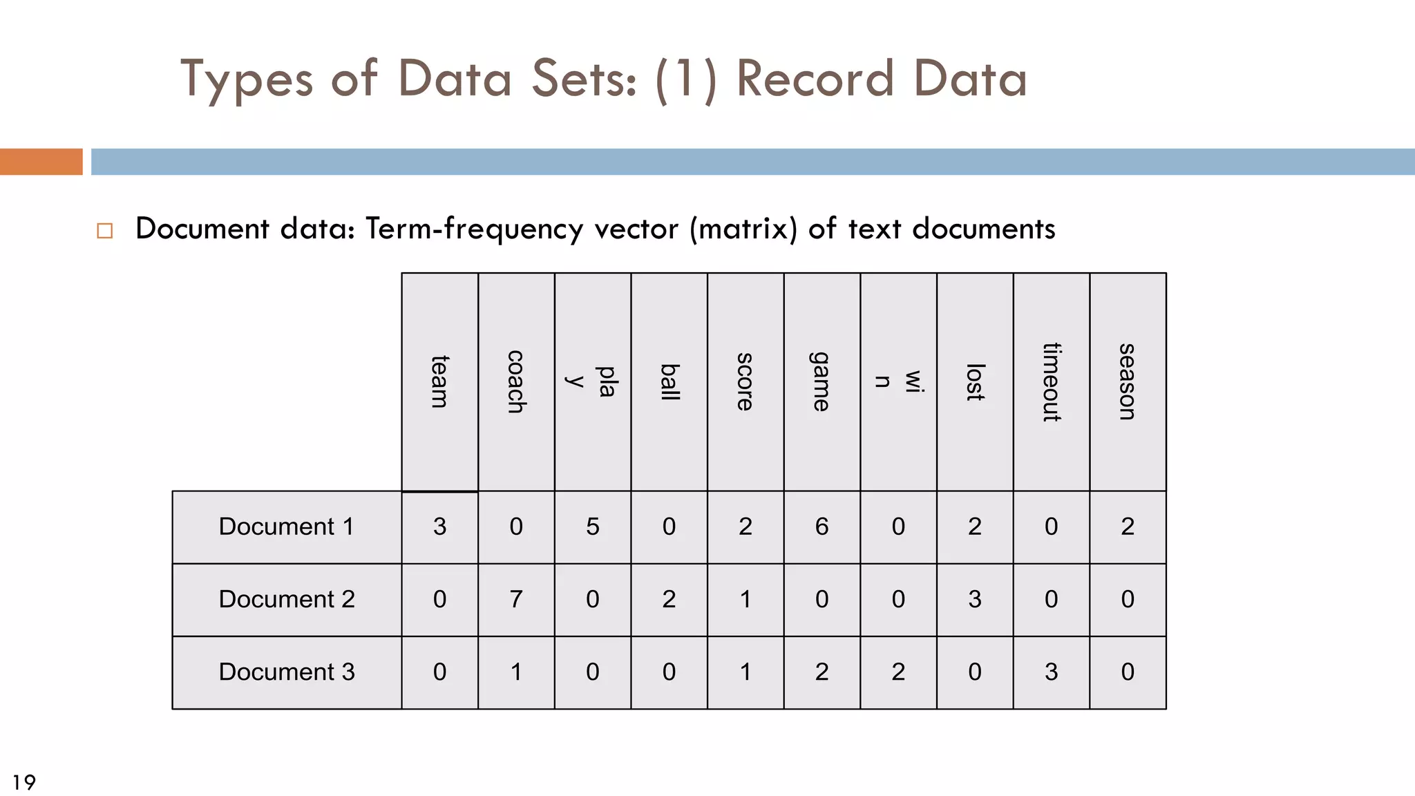
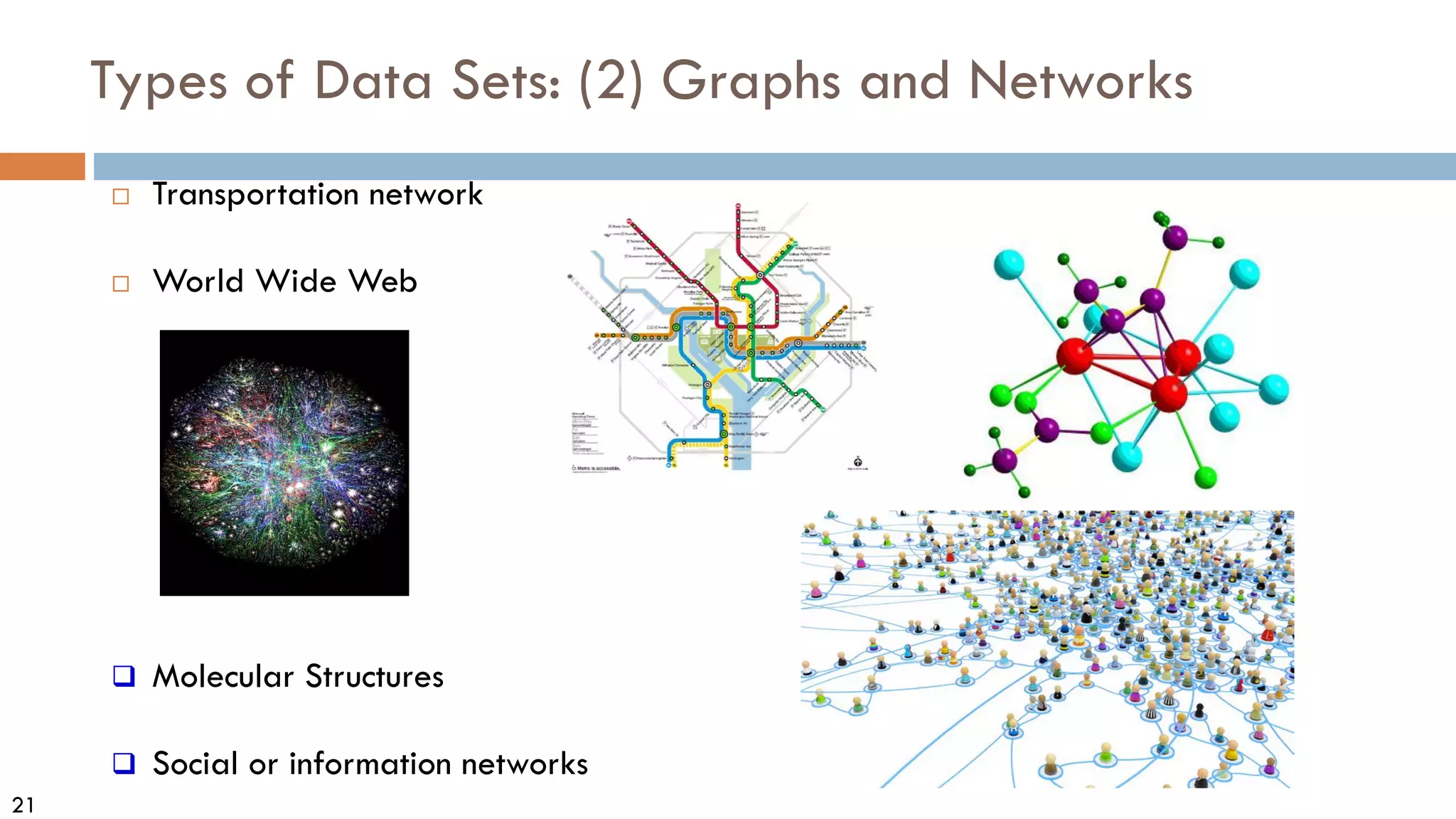
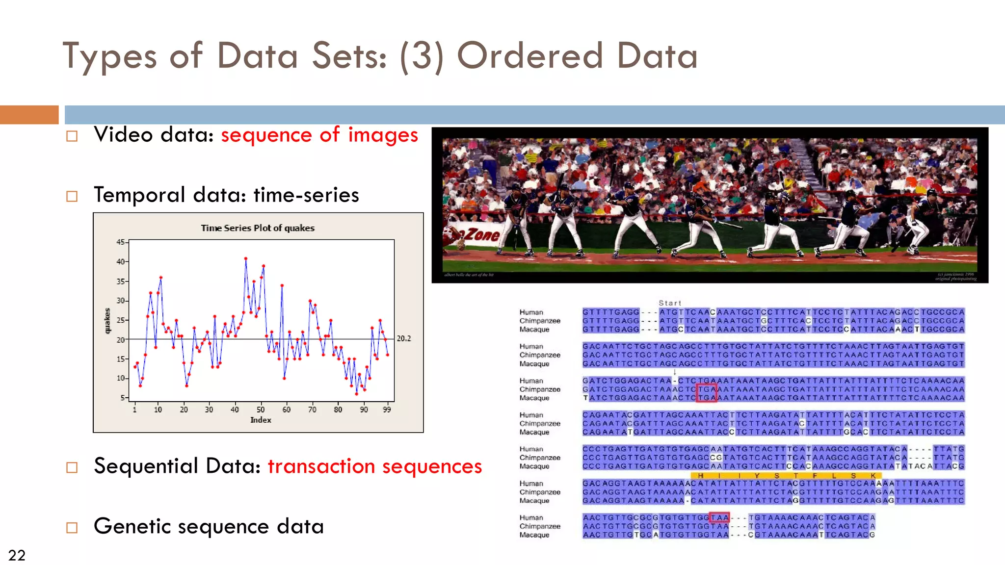
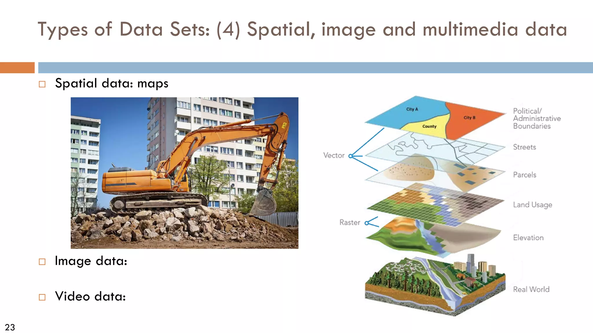
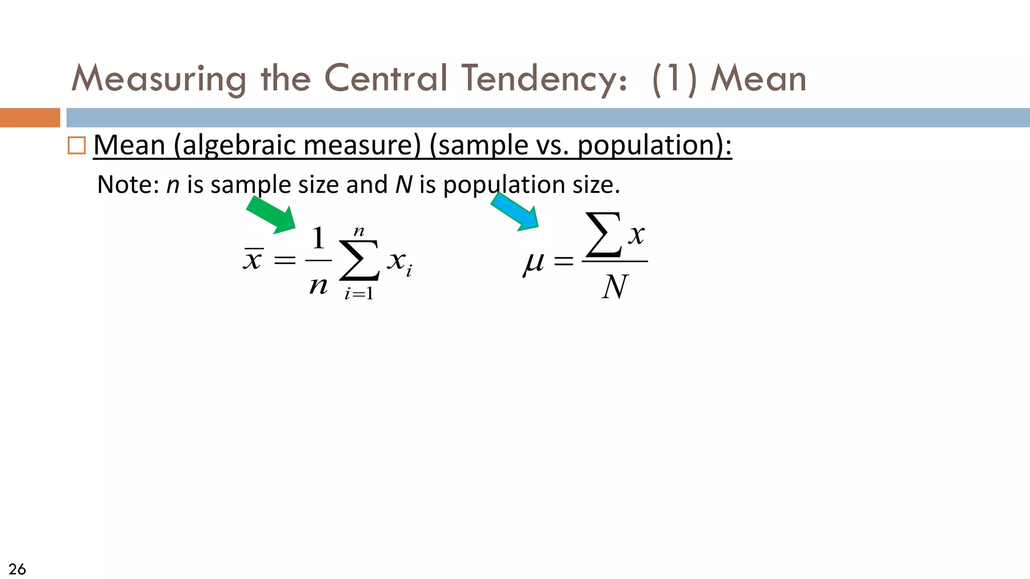
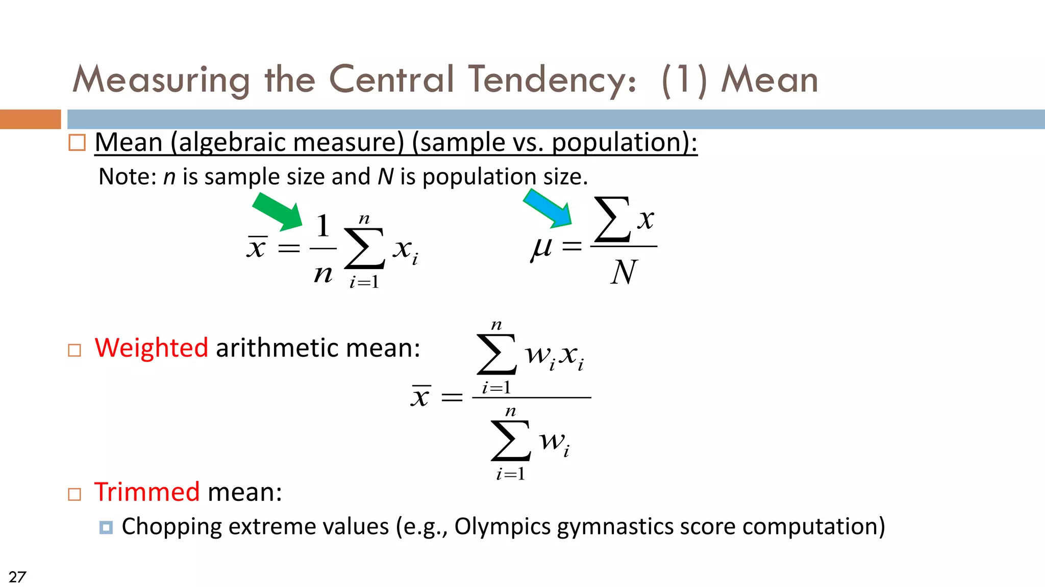
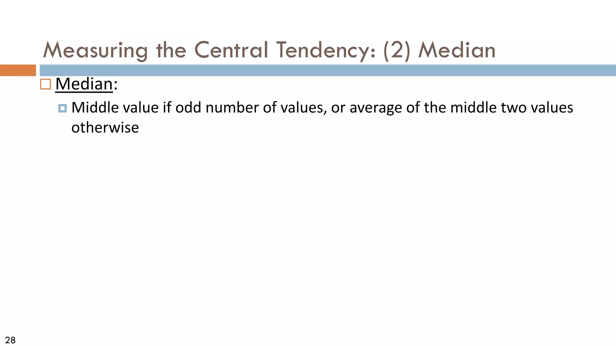
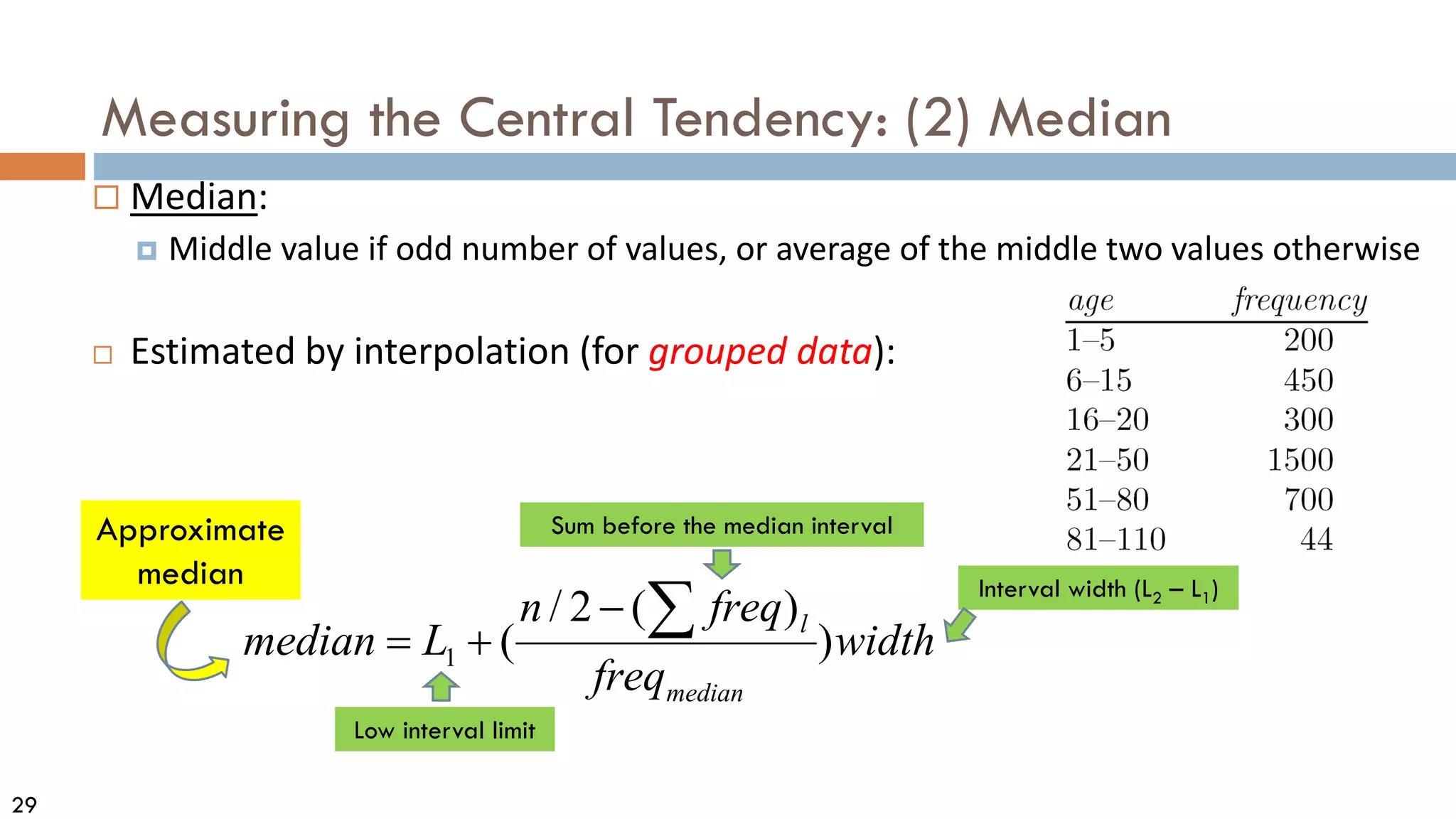
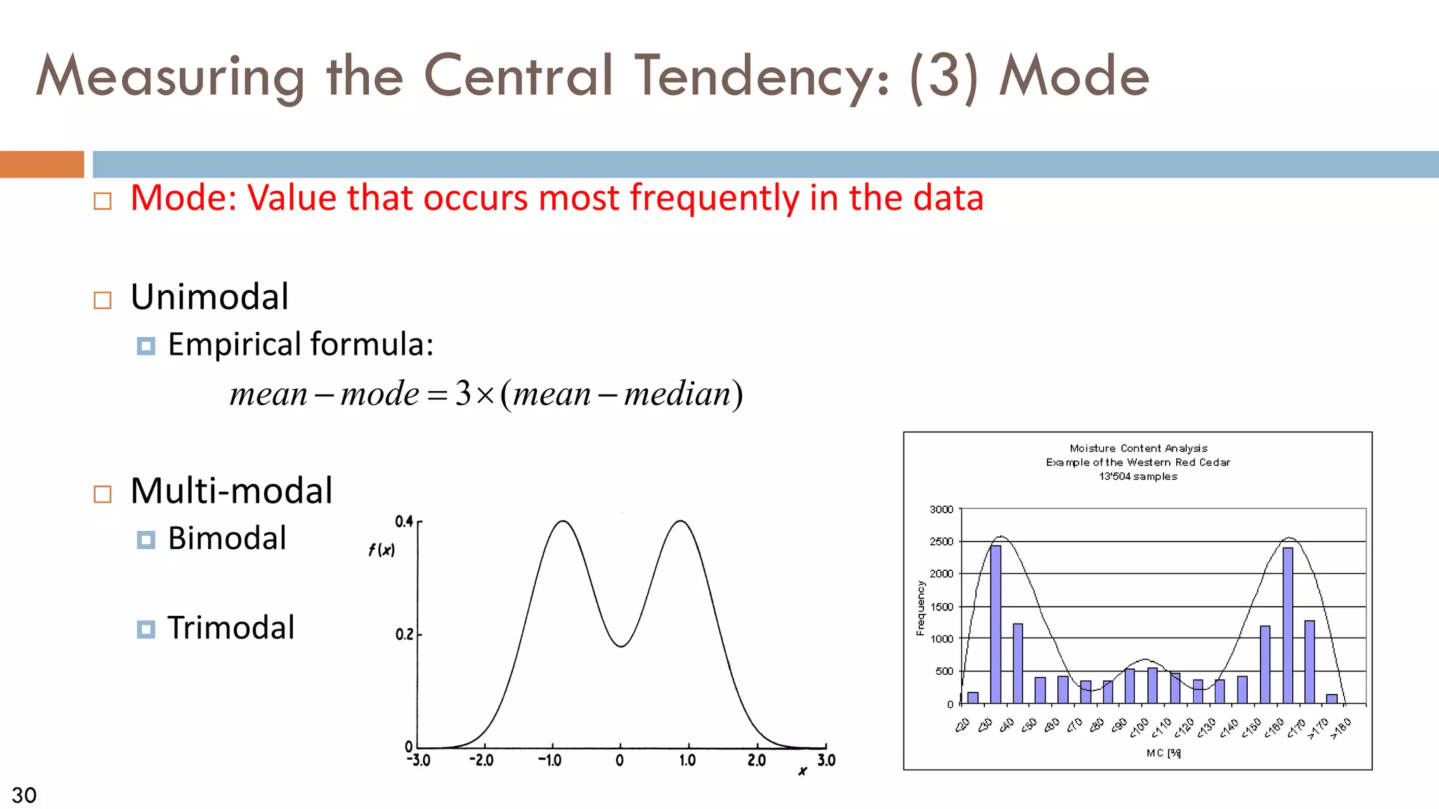
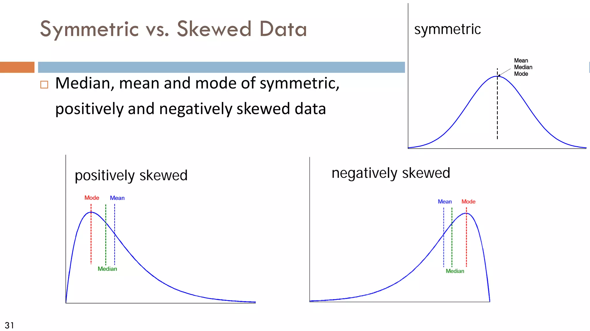
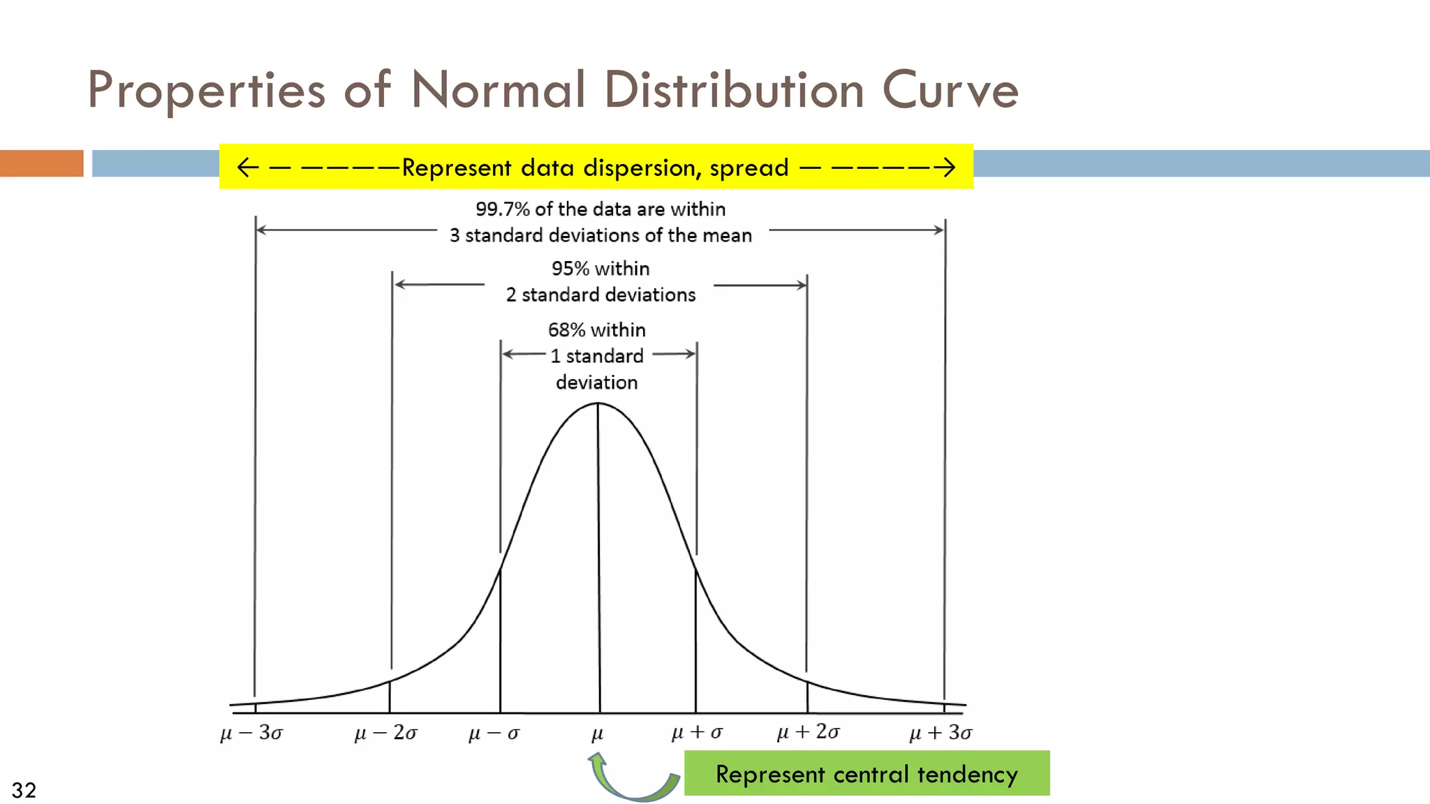
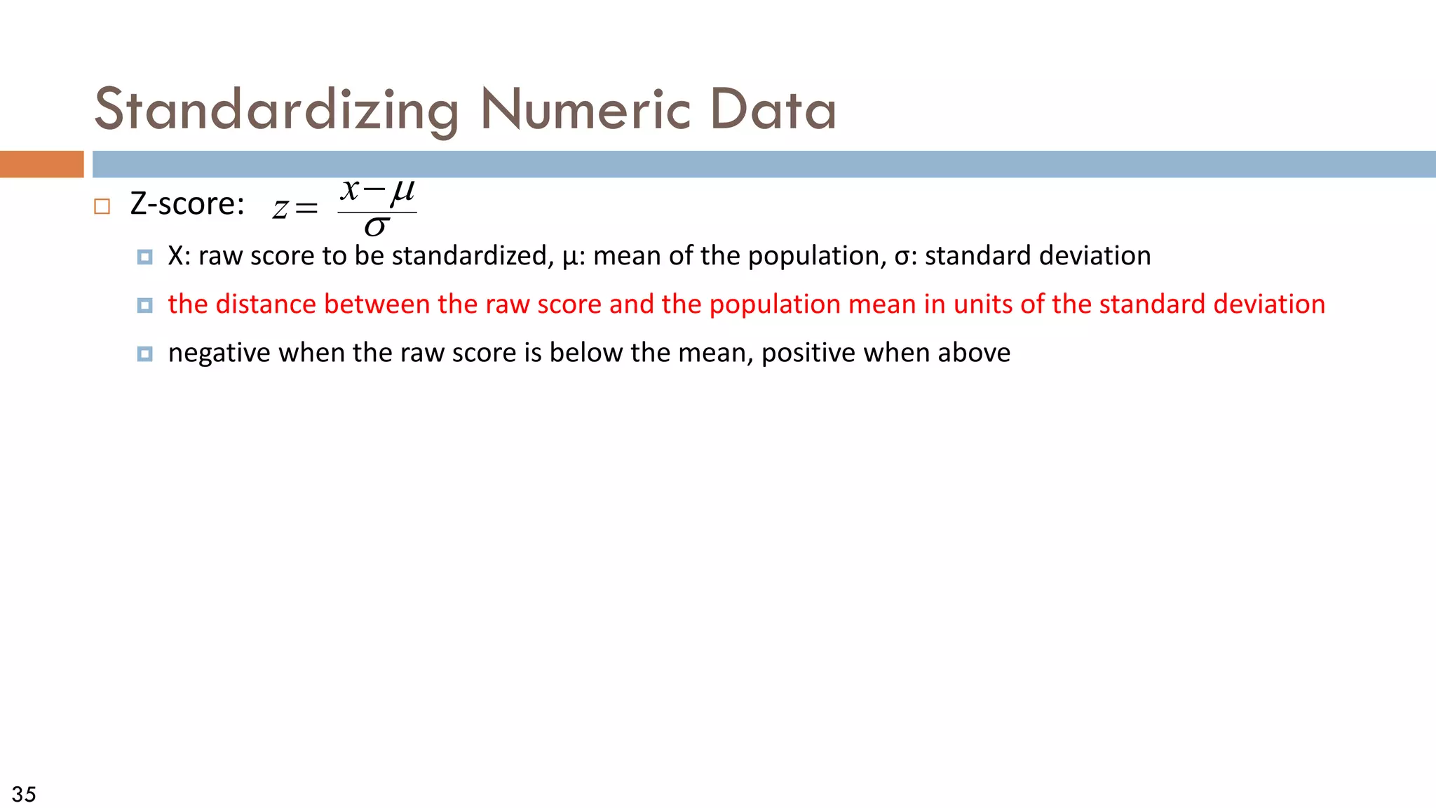
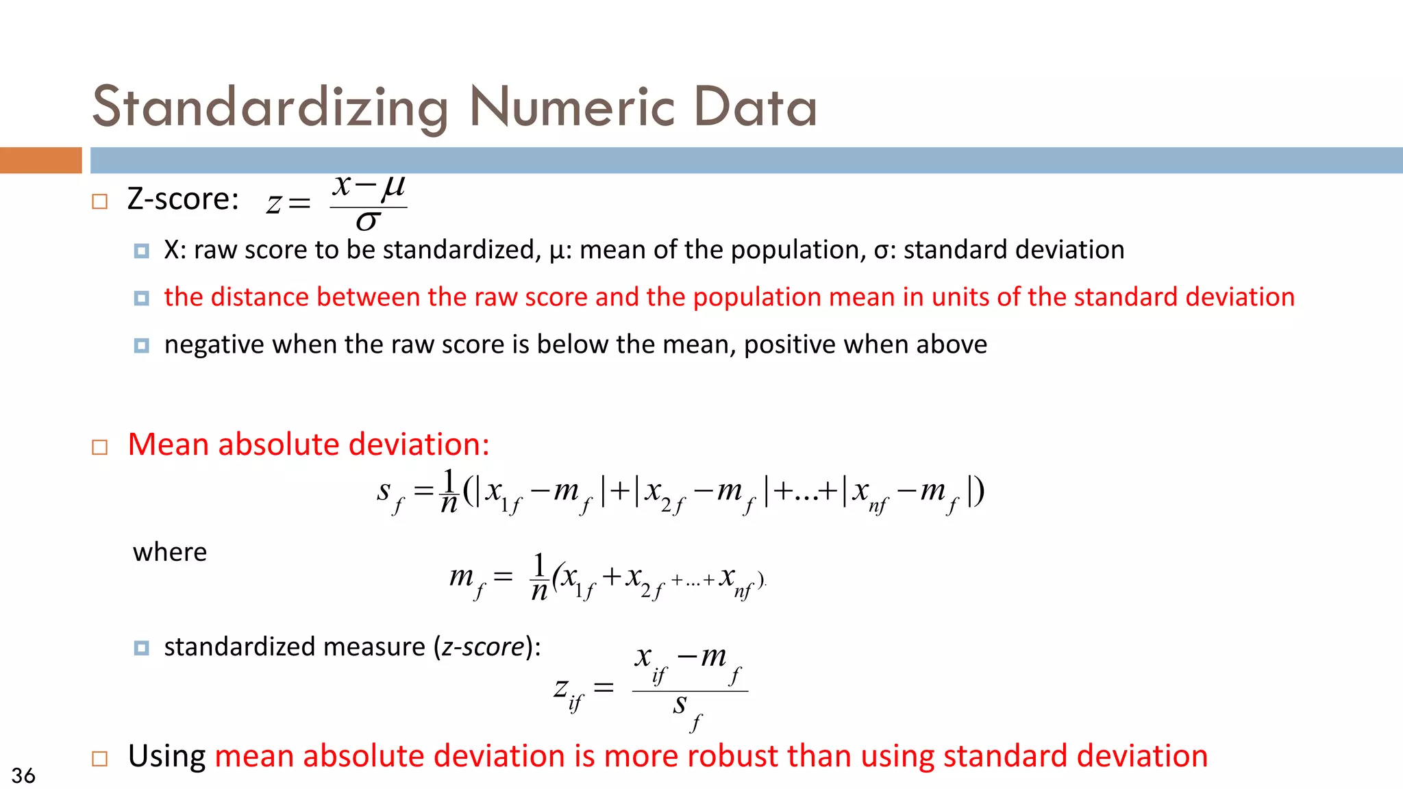
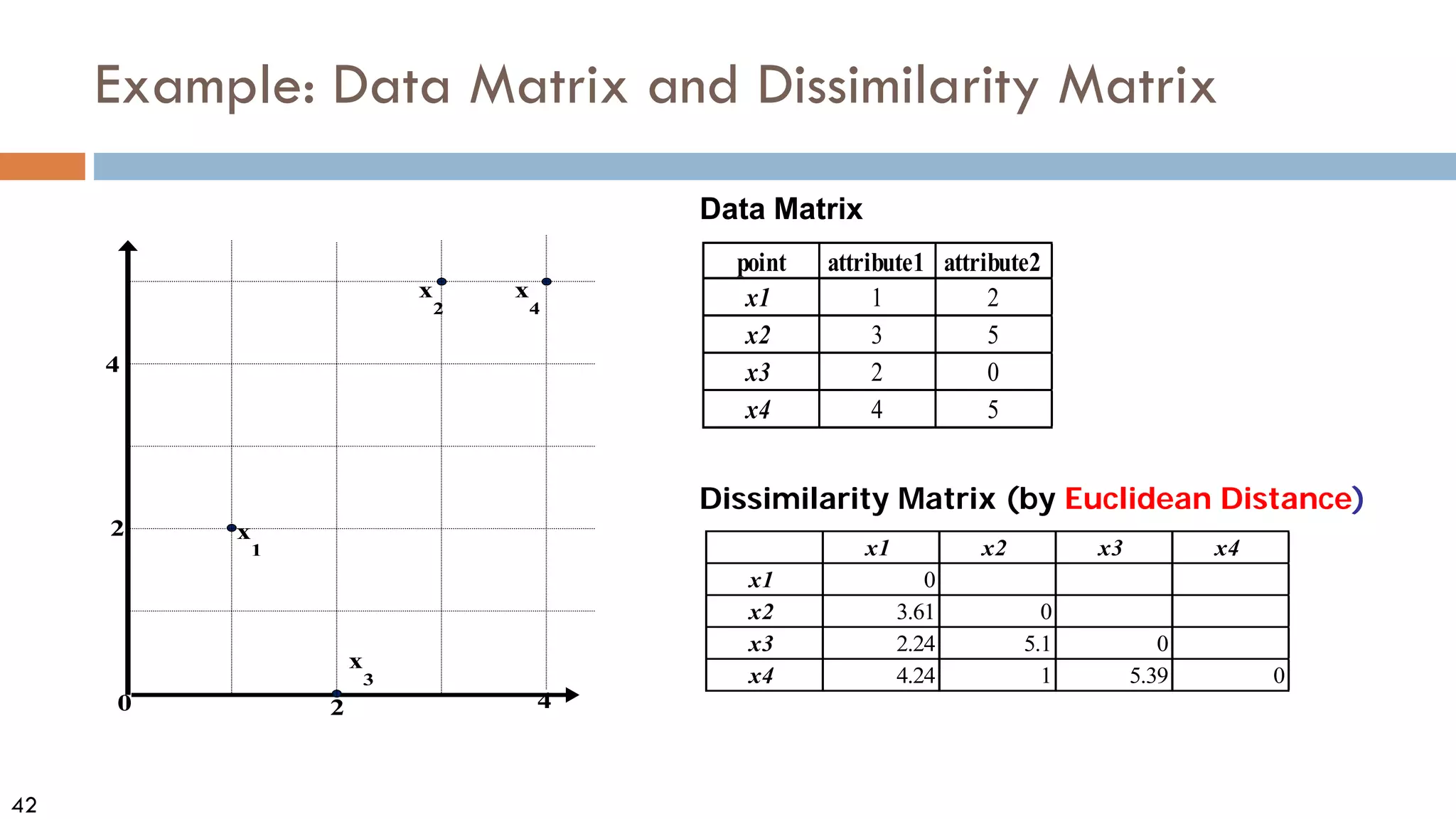
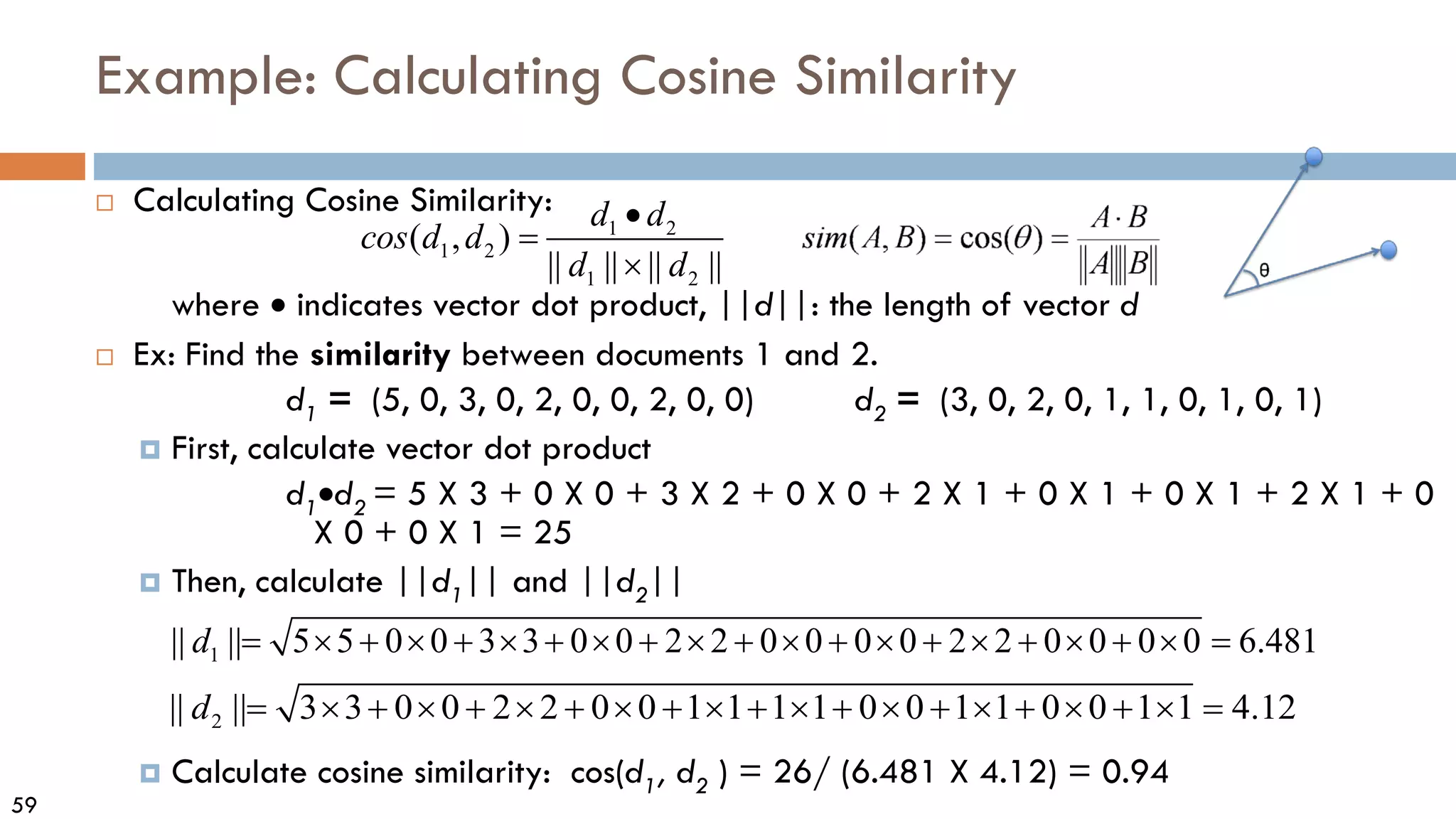
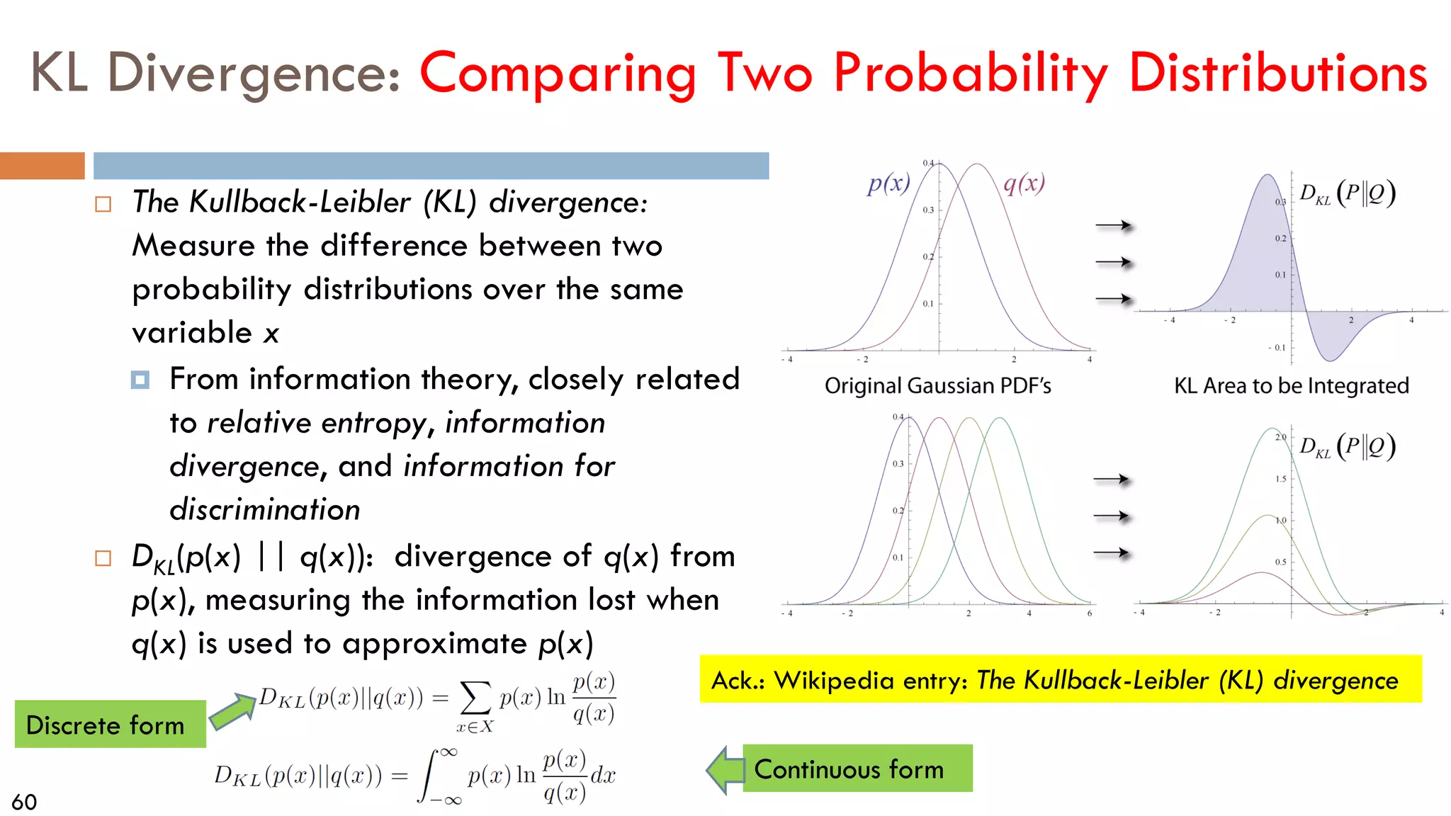
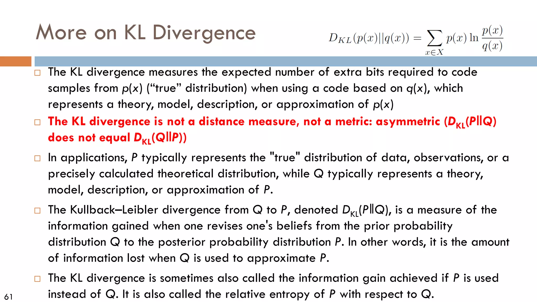
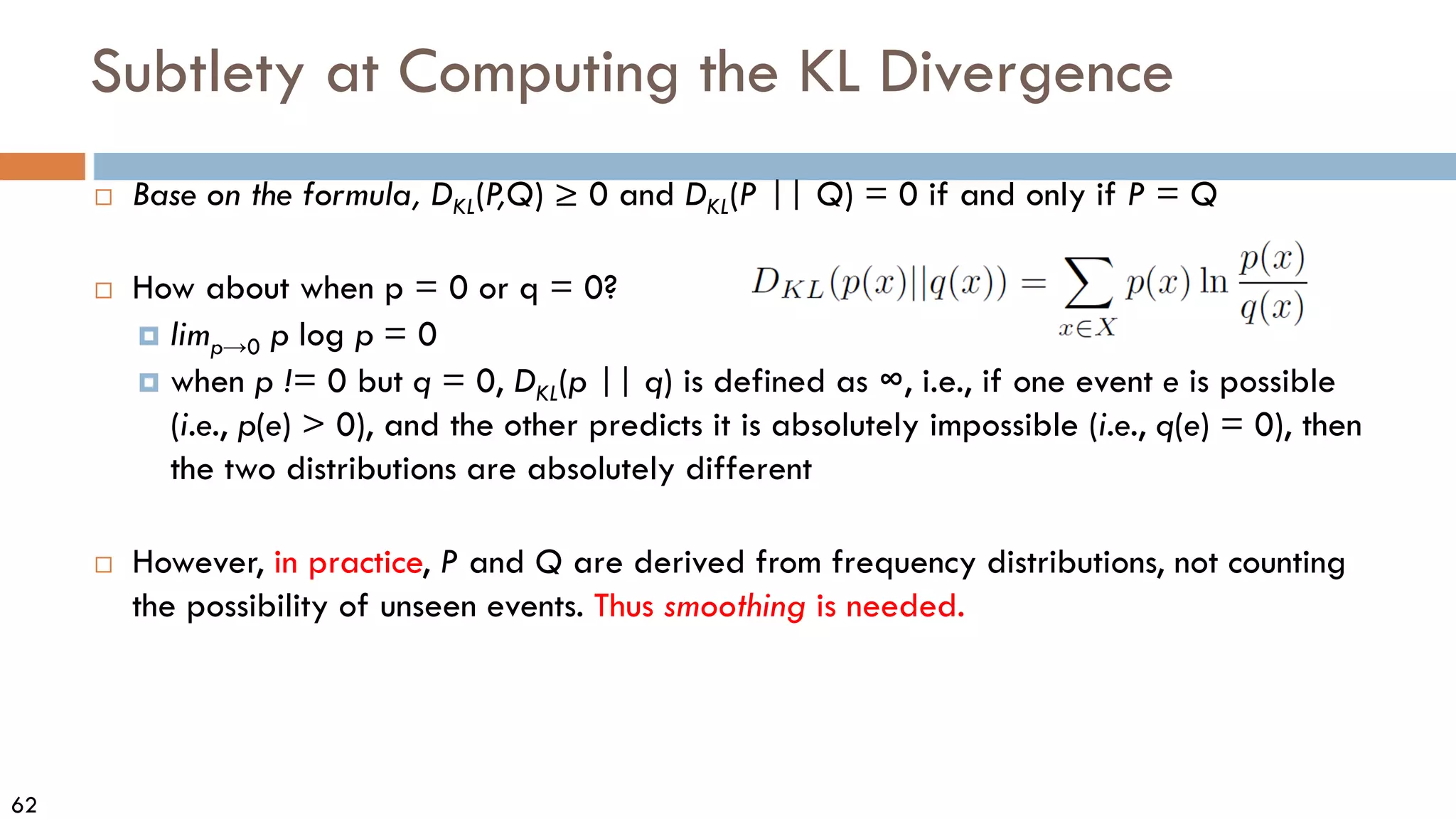
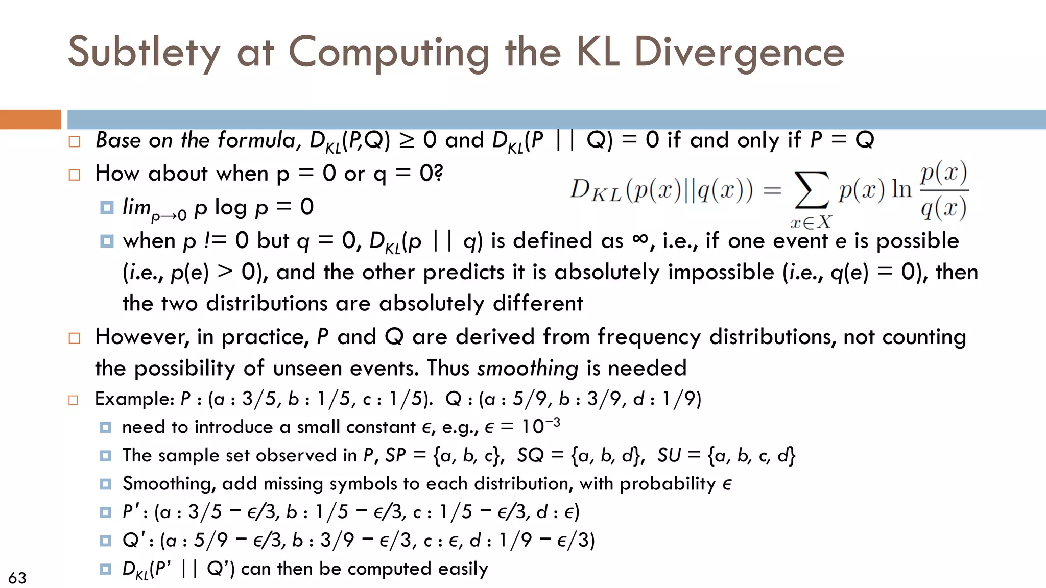
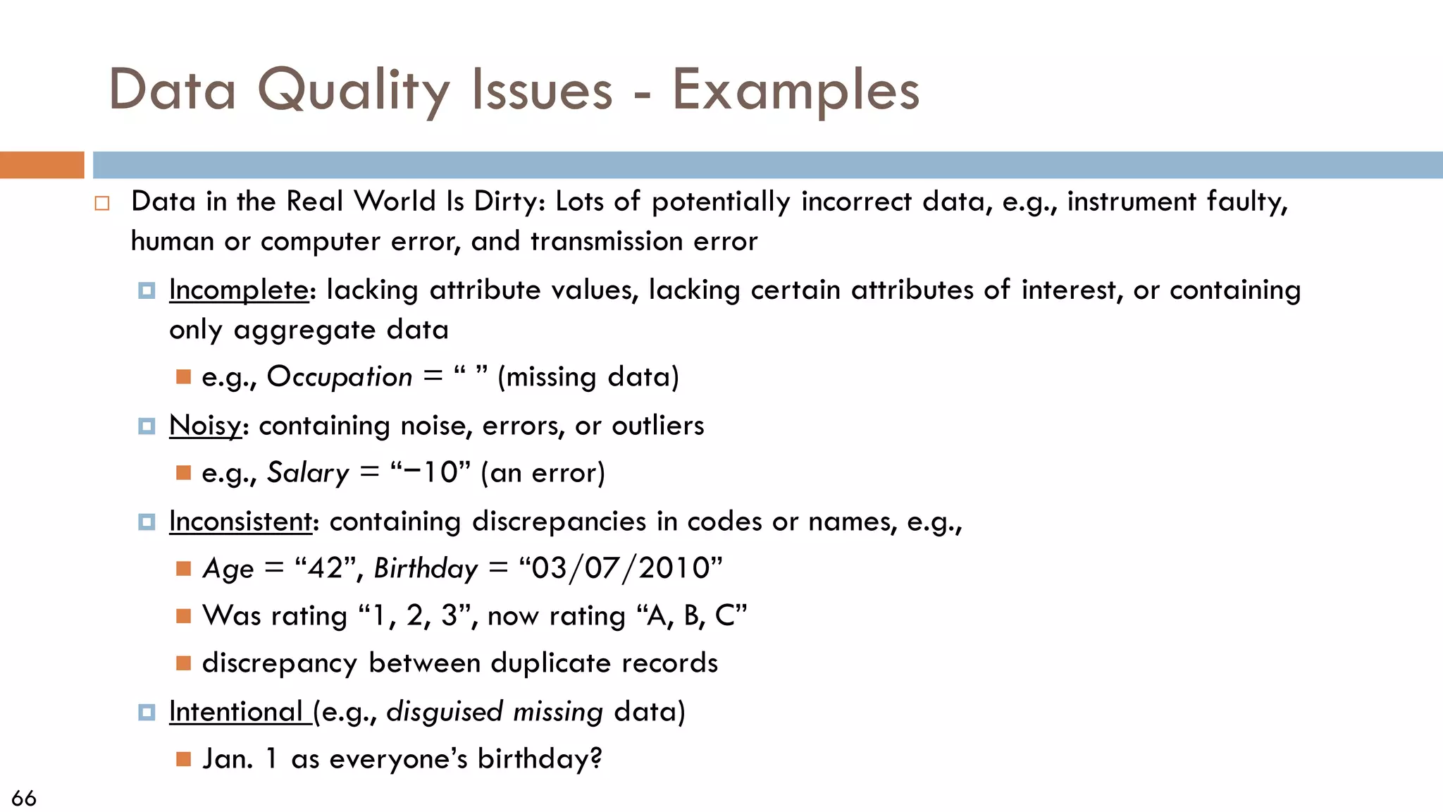
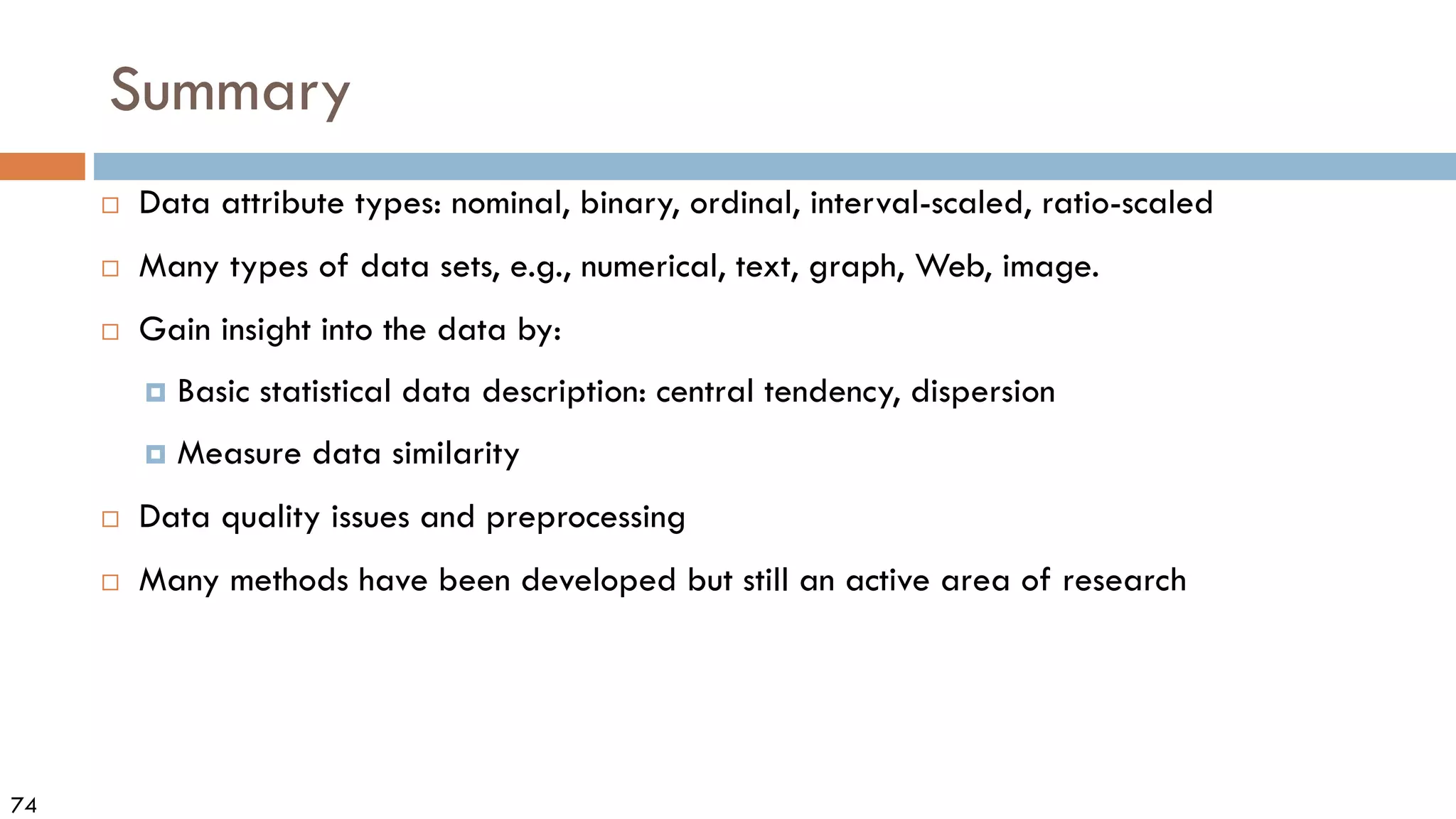
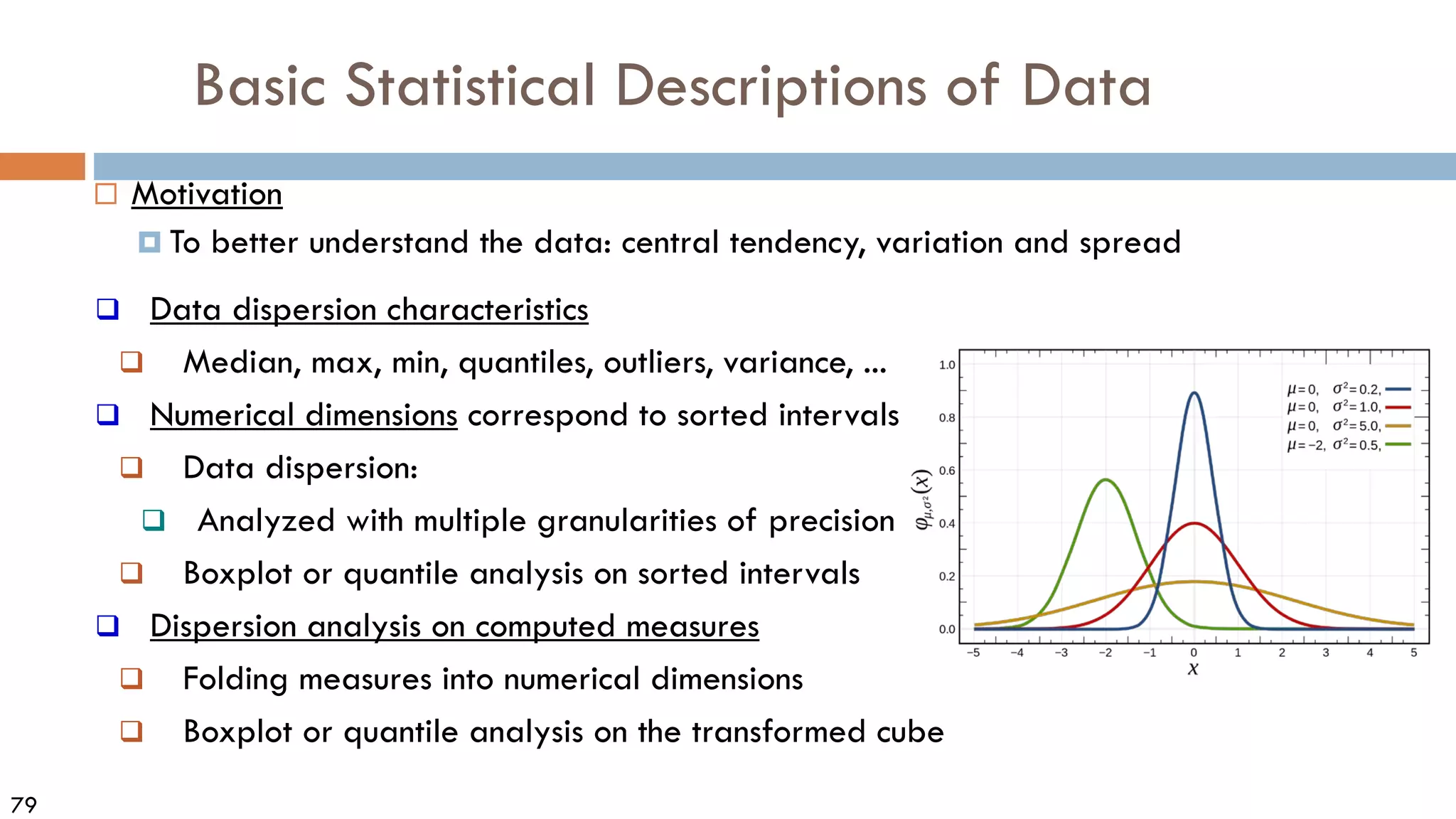
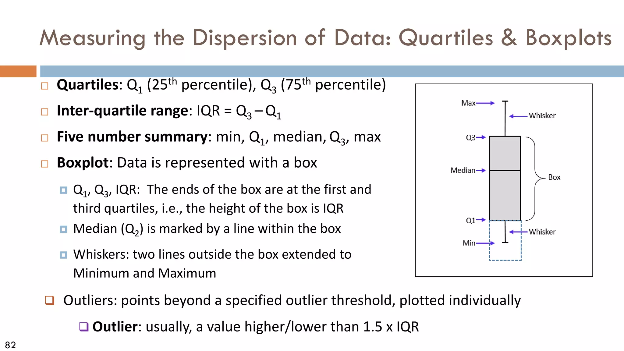
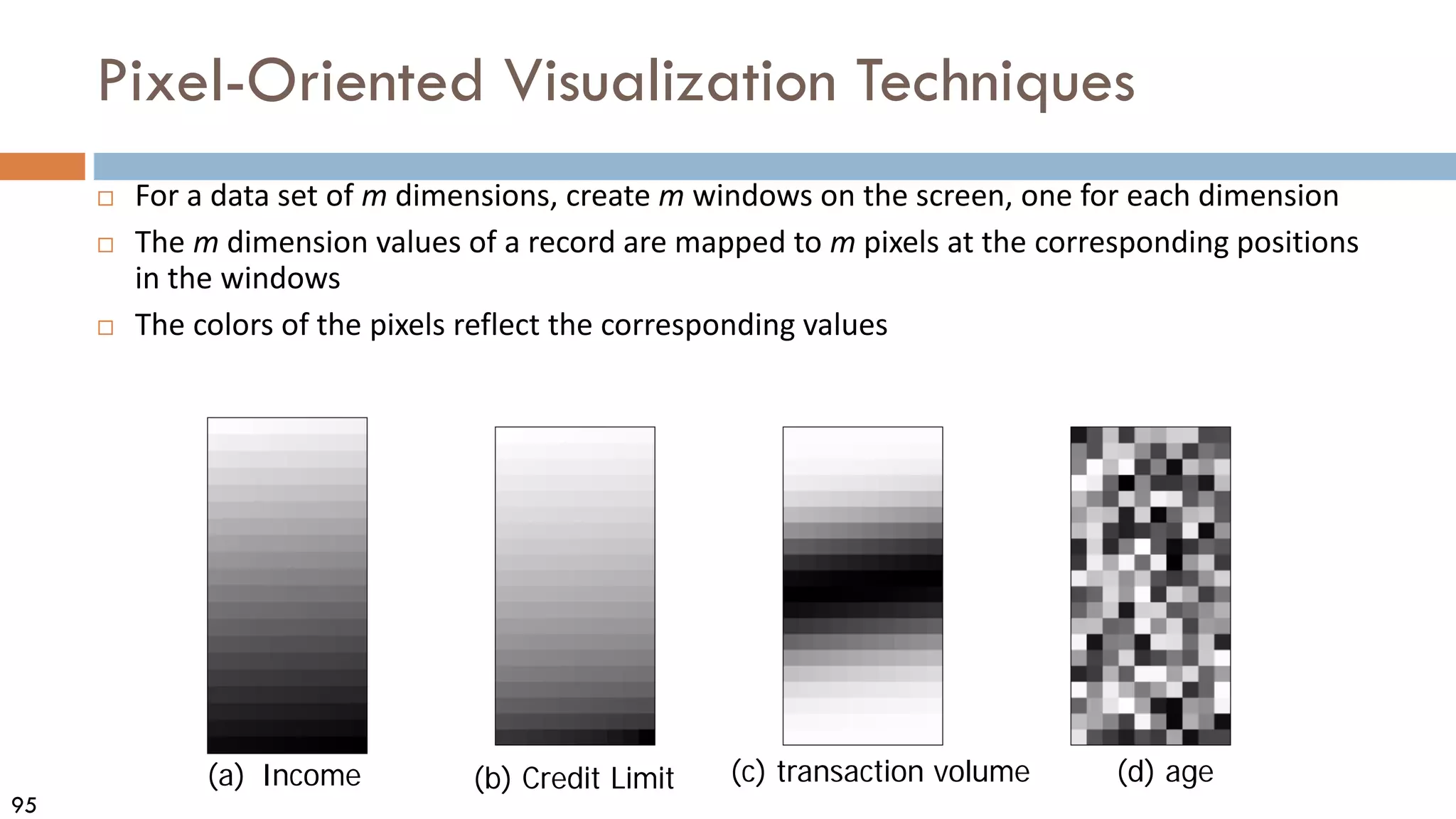
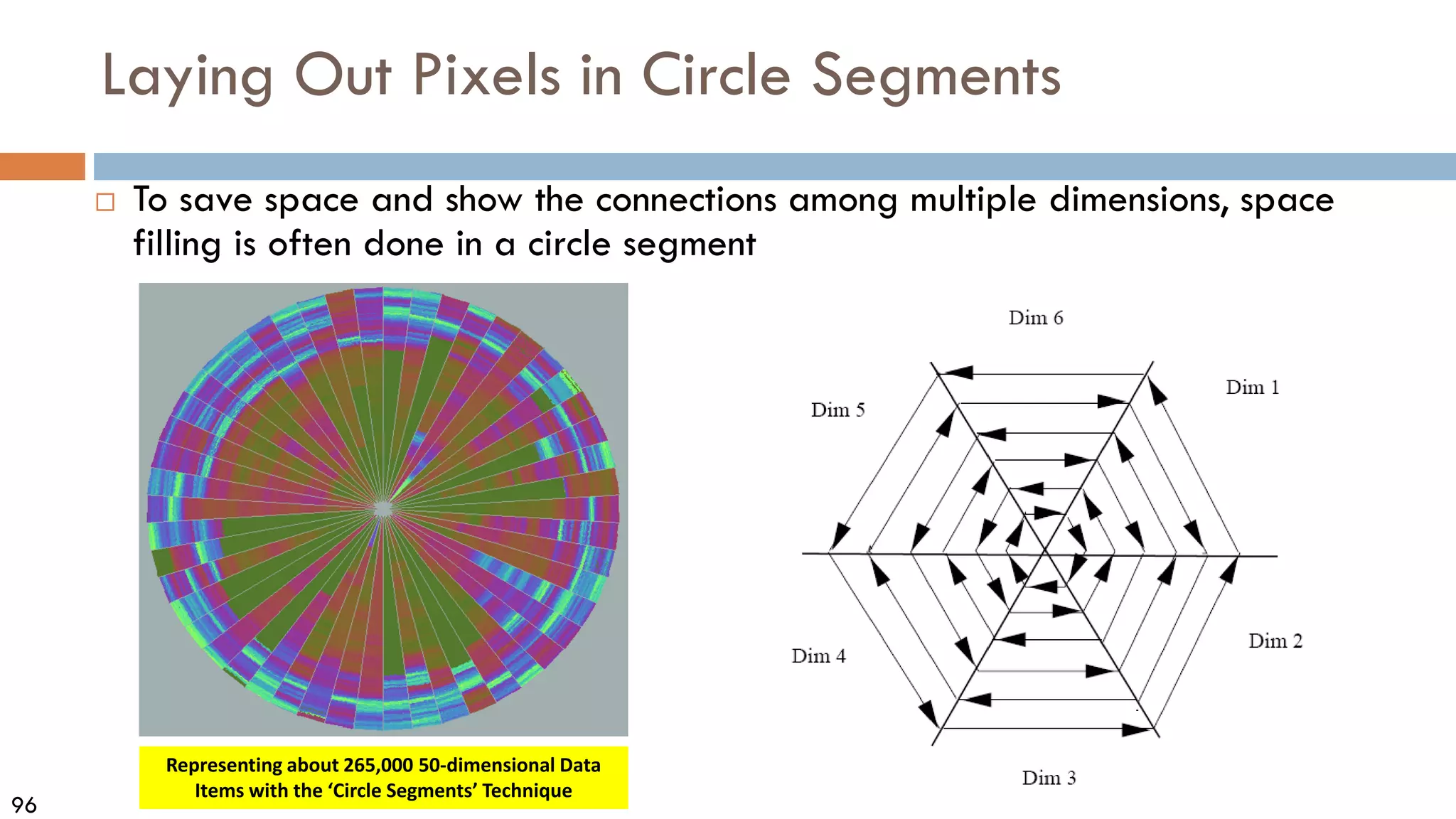
This document discusses data and data preprocessing in data mining. It defines what data is, including data objects and attributes. It describes different attribute types like nominal, binary, ordinal, interval-scaled and ratio-scaled numeric attributes. It also discusses measuring the central tendency of data using the mean, median and mode. Additionally, it covers measuring data distribution through variance, standard deviation and z-scores. Finally, it briefly introduces measuring data similarity and dissimilarity, as well as an overview of data preprocessing.

1. CSE5243 INTRO. TO DATA MINING
Data & Data Preprocessing
Huan Sun, CSE@The Ohio State University
Slides adapted from UIUC CS412, Fall 2017, by Prof. Jiawei Han

2. 2
Data & Data Preprocessing
 What is Data: Data Objects and Attribute Types
 Basic Statistical Descriptions of Data
 Measuring Data Similarity and Dissimilarity
 Data Preprocessing: An Overview
 Summary

3. 3
What is Data?
 Collection of data objects and their attributes

4. 4
What is Data?
 Collection of data objects and their attributes
Tid Refund Marital
Status
Taxable
Income Cheat
1 Yes Single 125K No
2 No Married 100K No
3 No Single 70K No
4 Yes Married 120K No
5 No Divorced 95K Yes
6 No Married 60K No
7 Yes Divorced 220K No
8 No Single 85K Yes
9 No Married 75K No
10 No Single 90K Yes
10
Attributes
Objects

5. 5
Data Objects
 Data sets are made up of data objects
 A data object represents an entity
 Examples:
 sales database: customers, store items, sales
 medical database: patients, treatments
 university database: students, professors, courses
 Also called samples , examples, instances, data points, objects, tuples

6. 6
Data Objects
 Data sets are made up of data objects
 A data object represents an entity
 Examples:
 sales database: customers, store items, sales
 medical database: patients, treatments
 university database: students, professors, courses
 Also called samples , examples, instances, data points, objects, tuples
 Data objects are described by attributes
 Database rows → data objects; columns → attributes

7. 7
Attributes
 Attribute (or dimensions, features, variables)
 A data field, representing a characteristic or feature of a data object.
 E.g., customer_ID, name, address
 Types:
 Nominal (e.g., red, blue)
 Binary (e.g., {true, false})
 Ordinal (e.g., {freshman, sophomore, junior, senior})
 Numeric: quantitative

8. 8
Attribute Types
 Nominal: categories, states, or “names of things”
 Hair_color = {auburn, black, blond, brown, grey, red, white}
 marital status, occupation, zip codes

9. 9
Attribute Types
 Nominal: categories, states, or “names of things”
 Hair_color = {auburn, black, blond, brown, grey, red, white}
 marital status, occupation, zip codes
 Binary
 Nominal attribute with only 2 states (0 and 1)
 Symmetric binary: both outcomes equally important
 e.g., gender
 Asymmetric binary: outcomes not equally important.
 e.g., medical test (positive vs. negative)
 Convention: assign 1 to most important outcome (e.g., HIV positive)

10. 10
Attribute Types
 Nominal: categories, states, or “names of things”
 Hair_color = {auburn, black, blond, brown, grey, red, white}
 marital status, occupation, ID numbers, zip codes
 Binary
 Nominal attribute with only 2 states (0 and 1)
 Symmetric binary: both outcomes equally important, e.g., gender
 Asymmetric binary: outcomes not equally important.
 e.g., medical test (positive vs. negative)
 Convention: assign 1 to most important outcome (e.g., HIV positive)
 Ordinal
 Values have a meaningful order (ranking) but magnitude between successive
values is not known
 Size = {small, medium, large}, grades, army rankings

11. 11
Numeric Attribute Types
 Quantity (integer or real-valued)
 Interval-scaled
 Measured on a scale of equal-sized units
 Values have order
 E.g., temperature in C˚or F˚, calendar dates
 No true zero-point

12. 12
Numeric Attribute Types
 Quantity (integer or real-valued)
 Interval-scaled
 Measured on a scale of equal-sized units
 Values have order
 E.g., temperature in C˚or F˚, calendar dates
 No true zero-point
 Ratio-scaled
 Inherent zero-point
 We can speak of values as being an order of magnitude larger than the unit
of measurement (10 K˚ is twice as high as 5 K˚).
 e.g., temperature in Kelvin, length, counts, monetary quantities

13. 13
 Q1: Is student ID a nominal, ordinal, or numerical attribute?
 Q2: What about eye color? Or color in the color spectrum of
physics?

14. 14
Discrete vs. Continuous Attributes
 Discrete Attribute
 Has only a finite or countably infinite set of values
 E.g., zip codes, profession, or the set of words in a collection of documents
 Sometimes, represented as integer variables
 Note: Binary attributes are a special case of discrete attributes

15. 15
Discrete vs. Continuous Attributes
 Discrete Attribute
 Has only a finite or countably infinite set of values
 Sometimes, represented as integer variables
 Note: Binary attributes are a special case of discrete attributes
 Continuous Attribute
 Has real numbers as attribute values
 E.g., temperature, height, or weight
 Practically, real values can only be measured and represented using a finite number
of digits
 Continuous attributes are typically represented as floating-point variables

16. 16
Types of Data Sets: (1) Record Data
 Relational records
 Relational tables, highly structured

17. 17
Types of Data Sets: (1) Record Data
 Data matrix, e.g., numerical matrix, crosstabs

18. 18
Types of Data Sets: (1) Record Data
 Transaction data

19. 19
Types of Data Sets: (1) Record Data
 Document data: Term-frequency vector (matrix) of text documents
Document 1
season
timeout
lost
wi
n
game
score
ball
pla
y
coach
team
Document 2
Document 3
3 0 5 0 2 6 0 2 0 2
0
0
7 0 2 1 0 0 3 0 0
1 0 0 1 2 2 0 3 0

20. 20
Types of Data Sets: (2) Graphs and Networks
 Transportation network
 World Wide Web

21. 21
Types of Data Sets: (2) Graphs and Networks
 Transportation network
 World Wide Web
 Molecular Structures
 Social or information networks

22. 22
Types of Data Sets: (3) Ordered Data
 Video data: sequence of images
 Temporal data: time-series
 Sequential Data: transaction sequences
 Genetic sequence data

23. 23
Types of Data Sets: (4) Spatial, image and multimedia data
 Spatial data: maps
 Image data:
 Video data:

24. 24
Chapter 2. Getting to Know Your Data
 Data Objects and Attribute Types
 Basic Statistical Descriptions of Data
 Measuring Data Similarity and Dissimilarity
 Data Preprocessing: An Overview
 Summary

25. 25
Basic Statistical Descriptions of Data
 Motivation
 To better understand the data: central tendency, variation and spread

26. 26
Measuring the Central Tendency: (1) Mean
 Mean (algebraic measure) (sample vs. population):
Note: n is sample size and N is population size.
N
x
∑
=
µ
∑
=
=
n
i
i
x
n
x
1
1

27. 27
Measuring the Central Tendency: (1) Mean
 Mean (algebraic measure) (sample vs. population):
Note: n is sample size and N is population size.
 Weighted arithmetic mean:
 Trimmed mean:
 Chopping extreme values (e.g., Olympics gymnastics score computation)
N
x
∑
=
µ
∑
=
=
n
i
i
x
n
x
1
1
∑
∑
=
=
= n
i
i
n
i
i
i
w
x
w
x
1
1

28. 28
Measuring the Central Tendency: (2) Median
 Median:
 Middle value if odd number of values, or average of the middle two values
otherwise

29. 29
Measuring the Central Tendency: (2) Median
 Median:
 Middle value if odd number of values, or average of the middle two values otherwise
 Estimated by interpolation (for grouped data):
width
freq
freq
n
L
median
median
l
)
)
(
2
/
(
1
∑
−
+
=
Approximate
median
Low interval limit
Interval width (L2 – L1)
Sum before the median interval

30. 30
Measuring the Central Tendency: (3) Mode
 Mode: Value that occurs most frequently in the data
 Unimodal
 Empirical formula:
 Multi-modal
 Bimodal
 Trimodal
)
(
3 median
mean
mode
mean −
×
=
−

31. 31
Symmetric vs. Skewed Data
 Median, mean and mode of symmetric,
positively and negatively skewed data
positively skewed negatively skewed
symmetric

32. 32
Properties of Normal Distribution Curve
← — ————Represent data dispersion, spread — ————→
Represent central tendency

33. 33
Measures Data Distribution: Variance and Standard Deviation
 Variance and standard deviation (sample: s, population: σ)
 Variance: (algebraic, scalable computation)
 Standard deviation s (or σ) is the square root of variance s2 (orσ2 )
∑
∑ =
=
−
=
−
=
n
i
i
n
i
i x
N
x
N 1
2
2
1
2
2 1
)
(
1
µ
µ
σ
∑ ∑
∑ = =
=
−
−
=
−
−
=
n
i
n
i
i
i
n
i
i x
n
x
n
x
x
n
s
1 1
2
2
1
2
2
]
)
(
1
[
1
1
)
(
1
1

34. 34
Measures Data Distribution: Variance and Standard Deviation
 Variance and standard deviation (sample: s, population: σ)
 Variance: (algebraic, scalable computation)
 Standard deviation s (or σ) is the square root of variance s2 (orσ2 )
∑
∑ =
=
−
=
−
=
n
i
i
n
i
i x
N
x
N 1
2
2
1
2
2 1
)
(
1
µ
µ
σ
∑ ∑
∑ = =
=
−
−
=
−
−
=
n
i
n
i
i
i
n
i
i x
n
x
n
x
x
n
s
1 1
2
2
1
2
2
]
)
(
1
[
1
1
)
(
1
1
?

35. 35
Standardizing Numeric Data
 Z-score:
 X: raw score to be standardized, μ: mean of the population, σ: standard deviation
 the distance between the raw score and the population mean in units of the standard deviation
 negative when the raw score is below the mean, positive when above
σ
µ
−
= x
z

36. 36
Standardizing Numeric Data
 Z-score:
 X: raw score to be standardized, μ: mean of the population, σ: standard deviation
 the distance between the raw score and the population mean in units of the standard deviation
 negative when the raw score is below the mean, positive when above
 Mean absolute deviation:
where
 standardized measure (z-score):
 Using mean absolute deviation is more robust than using standard deviation
σ
µ
−
= x
z
.
)
...
2
1
1
nf
f
f
f
x
x
(x
n
m +
+
+
=
|)
|
...
|
|
|
(|
1
2
1 f
nf
f
f
f
f
f
m
x
m
x
m
x
n
s −
+
+
−
+
−
=
f
f
if
if s
m
x
z
−
=

37. 37
Data & Data Preprocessing
 Data Objects and Attribute Types
 Basic Statistical Descriptions of Data
 Measuring Data Similarity and Dissimilarity
 Data Preprocessing: An Overview
 Summary

38. 38
Similarity, Dissimilarity, and Proximity
 Similarity measure or similarity function
 A real-valued function that quantifies the similarity between two objects
 Measure how two data objects are alike: The higher value, the more alike
 Often falls in the range [0,1]: 0: no similarity; 1: completely similar

39. 39
Similarity, Dissimilarity, and Proximity
 Similarity measure or similarity function
 A real-valued function that quantifies the similarity between two objects
 Measure how two data objects are alike: The higher value, the more alike
 Often falls in the range [0,1]: 0: no similarity; 1: completely similar
 Dissimilarity (or distance) measure
 Numerical measure of how different two data objects are
 In some sense, the inverse of similarity: The lower, the more alike
 Minimum dissimilarity is often 0 (i.e., completely similar)
 Range [0, 1] or [0, ∞) , depending on the definition
 Proximity usually refers to either similarity or dissimilarity

40. 40
Data Matrix and Dissimilarity Matrix
 Data matrix
 A data matrix of n data points with l dimensions
11 12 1
21 22 2
1 2
...
...
...
l
l
n n nl
x x x
x x x
D
x x x
 
 
 
=
 
 
 
   

41. 41
Data Matrix and Dissimilarity Matrix
 Data matrix
 A data matrix of n data points with l dimensions
 Dissimilarity (distance) matrix
 n data points, but registers only the distance d(i, j)
(typically metric)
 Usually symmetric
 Distance functions are usually different for real, boolean,
categorical, ordinal, ratio, and vector variables
 Weights can be associated with different variables based
on applications and data semantics
11 12 1
21 22 2
1 2
...
...
...
l
l
n n nl
x x x
x x x
D
x x x
 
 
 
=
 
 
 
   
0
(2,1) 0
( ,1) ( ,2) ... 0
d
d n d n
 
 
 
 
 
 
  

42. 42
Example: Data Matrix and Dissimilarity Matrix
point attribute1 attribute2
x1 1 2
x2 3 5
x3 2 0
x4 4 5
Dissimilarity Matrix (by Euclidean Distance)
x1 x2 x3 x4
x1 0
x2 3.61 0
x3 2.24 5.1 0
x4 4.24 1 5.39 0
Data Matrix
0 2 4
2
4
x
1
x
2
x
3
x
4

43. 43
Distance on Numeric Data: Minkowski Distance
 Minkowski distance: A popular distance measure
where i = (xi1, xi2, …, xil) and j = (xj1, xj2, …, xjl) are two l-dimensional data
objects, and p is the order (the distance so defined is also called L-p norm)
1 1 2 2
( , ) | | | | | |
p p p
p
i j i j il jl
d i j x x x x x x
= − + − + + −


44. 44
Distance on Numeric Data: Minkowski Distance
 Minkowski distance: A popular distance measure
where i = (xi1, xi2, …, xil) and j = (xj1, xj2, …, xjl) are two l-dimensional data
objects, and p is the order (the distance so defined is also called L-p norm)
 Properties
 d(i, j) > 0 if i ≠ j, and d(i, i) = 0 (Positivity)
 d(i, j) = d(j, i) (Symmetry)
 d(i, j) ≤ d(i, k) + d(k, j) (Triangle Inequality)
 A distance that satisfies these properties is a metric
 Note: There are nonmetric dissimilarities, e.g., set differences
1 1 2 2
( , ) | | | | | |
p p p
p
i j i j il jl
d i j x x x x x x
= − + − + + −


45. 45
Special Cases of Minkowski Distance
 p = 1: (L1 norm) Manhattan (or city block) distance
 E.g., the Hamming distance: the number of bits that are different
between two binary vectors
1 1 2 2
( , ) | | | | | |
i j i j il jl
d i j x x x x x x
= − + − + + −


46. 46
Special Cases of Minkowski Distance
 p = 1: (L1 norm) Manhattan (or city block) distance
 E.g., the Hamming distance: the number of bits that are different
between two binary vectors
 p = 2: (L2 norm) Euclidean distance
2 2 2
1 1 2 2
( , ) | | | | | |
i j i j il jl
d i j x x x x x x
= − + − + + −

1 1 2 2
( , ) | | | | | |
i j i j il jl
d i j x x x x x x
= − + − + + −


47. 47
Special Cases of Minkowski Distance
 p = 1: (L1 norm) Manhattan (or city block) distance
 E.g., the Hamming distance: the number of bits that are different
between two binary vectors
 p = 2: (L2 norm) Euclidean distance
 p → ∞: (Lmax norm, L∞ norm) “supremum” distance
 The maximum difference between any component (attribute) of the
vectors
2 2 2
1 1 2 2
( , ) | | | | | |
i j i j il jl
d i j x x x x x x
= − + − + + −

1 1 2 2
( , ) | | | | | |
i j i j il jl
d i j x x x x x x
= − + − + + −

1 1 2 2
1
( , ) lim | | | | | | | |
max
l
p p p
p
i j i j il jl if if
p f
d i j x x x x x x x x
→∞ =
= − + − + + − = −


48. 48
Example: Minkowski Distance at Special Cases
point attribute 1 attribute 2
x1 1 2
x2 3 5
x3 2 0
x4 4 5
L x1 x2 x3 x4
x1 0
x2 5 0
x3 3 6 0
x4 6 1 7 0
L2 x1 x2 x3 x4
x1 0
x2 3.61 0
x3 2.24 5.1 0
x4 4.24 1 5.39 0
L∞ x1 x2 x3 x4
x1 0
x2 3 0
x3 2 5 0
x4 3 1 5 0
Manhattan
(L1)
Euclidean
(L2)
Supremum
(L∞)
0 2 4
2
4
x
1
x
2
x
3
x
4

49. 49
Proximity Measure for Binary Attributes
 A contingency table for binary data
 Distance measure for symmetric binary variables:
 Distance measure for asymmetric binary variables:
Object i
Object j

50. 50
Proximity Measure for Binary Attributes
 A contingency table for binary data
 Distance measure for symmetric binary variables:
 Distance measure for asymmetric binary variables:
 Jaccard coefficient (similarity measure for asymmetric
binary variables):
 Note: Jaccard coefficient is the same as “coherence”:
Object i
Object j
(a concept discussed in Pattern Discovery)

51. 51
Example: Dissimilarity between Asymmetric Binary Variables
 Gender is a symmetric attribute (not counted in)
 The remaining attributes are asymmetric binary
 Let the values Y and P be 1, and the value N be 0
Name Gender Fever Cough Test-1 Test-2 Test-3 Test-4
Jack M Y N P N N N
Mary F Y N P N P N
Jim M Y P N N N N

52. 52
Example: Dissimilarity between Asymmetric Binary Variables
 Gender is a symmetric attribute (not counted in)
 The remaining attributes are asymmetric binary
 Let the values Y and P be 1, and the value N be 0
Name Gender Fever Cough Test-1 Test-2 Test-3 Test-4
Jack M Y N P N N N
Mary F Y N P N P N
Jim M Y P N N N N
1 0 ∑row
1 2 0 2
0 1 3 4
∑co
l
3 3 6
Jack
Mary
1 0 ∑row
1 1 1 2
0 1 3 4
∑co
l
2 4 6
Jim
1 0 ∑row
1 1 1 2
0 2 2 4
∑col 3 3 6
Jim
Mary
Jack
Contingency table

53. 53
Example: Dissimilarity between Asymmetric Binary Variables
 Gender is a symmetric attribute (not counted in)
 The remaining attributes are asymmetric binary
 Let the values Y and P be 1, and the value N be 0
 Distance:
Name Gender Fever Cough Test-1 Test-2 Test-3 Test-4
Jack M Y N P N N N
Mary F Y N P N P N
Jim M Y P N N N N
75
.
0
2
1
1
2
1
)
,
(
67
.
0
1
1
1
1
1
)
,
(
33
.
0
1
0
2
1
0
)
,
(
=
+
+
+
=
=
+
+
+
=
=
+
+
+
=
mary
jim
d
jim
jack
d
mary
jack
d
1 0 ∑row
1 2 0 2
0 1 3 4
∑co
l
3 3 6
Jack
Mary
1 0 ∑row
1 1 1 2
0 1 3 4
∑co
l
2 4 6
Jim
1 0 ∑row
1 1 1 2
0 2 2 4
∑col 3 3 6
Jim
Mary
Jack
Contingency table

54. 54
Proximity Measure for Categorical Attributes
 Categorical data, also called nominal attributes
 Example: Color (red, yellow, blue, green), profession, etc.
 Method 1: Simple matching
 m: # of matches, p: total # of variables
 Method 2: Use a large number of binary attributes
 Creating a new binary attribute for each of the M nominal states
p
m
p
j
i
d −
=
)
,
(

55. 55
Ordinal Variables
 An ordinal variable can be discrete or continuous
 Order is important, e.g., rank (e.g., freshman, sophomore, junior, senior)
 Can be treated like interval-scaled
 Replace an ordinal variable value by its rank:
 Map the range of each variable onto [0, 1] by replacing i-th object in
the f-th variable by
 Example: freshman: 0; sophomore: 1/3; junior: 2/3; senior 1
 Then distance: d(freshman, senior) = 1, d(junior, senior) = 1/3
 Compute the dissimilarity using methods for interval-scaled variables
1
1
if
if
f
r
z
M
−
=
−
{1,..., }
if f
r M
∈

56. 56
Attributes of Mixed Type
 A dataset may contain all attribute types
 Nominal, symmetric binary, asymmetric binary, numeric, and ordinal
 One may use a weighted formula to combine their effects:
 If f is numeric: Use the normalized distance
 If f is binary or nominal: dij
(f) = 0 if xif = xjf; or dij
(f) = 1 otherwise
 If f is ordinal
 Compute ranks zif (where )
 Treat zif as interval-scaled
1
1
if
if
f
r
z
M
−
=
−
( ) ( )
1
( )
1
( , )
p
f f
ij ij
f
p
f
ij
f
w d
d i j
w
=
=
=
∑
∑

57. 57
Cosine Similarity of Two Vectors
 A document can be represented by a bag of terms or a long vector, with each attribute
recording the frequency of a particular term (such as word, keyword, or phrase) in the
document
 Other vector objects: Gene features in micro-arrays
 Applications: Information retrieval, biologic taxonomy, gene feature mapping, etc.
 Cosine measure: If d1 and d2 are two vectors (e.g., term-frequency vectors), then
where • indicates vector dot product, ||d||: the length of vector d
1 2
1 2
1 2
( , )
|| || || ||
d d
cos d d
d d
•
=
×

58. 58
Example: Calculating Cosine Similarity
 Calculating Cosine Similarity:
where • indicates vector dot product, ||d||: the length of vector d
1 2
1 2
1 2
( , )
|| || || ||
d d
cos d d
d d
•
=
×

59. 59
Example: Calculating Cosine Similarity
 Calculating Cosine Similarity:
where • indicates vector dot product, ||d||: the length of vector d
 Ex: Find the similarity between documents 1 and 2.
d1 = (5, 0, 3, 0, 2, 0, 0, 2, 0, 0) d2 = (3, 0, 2, 0, 1, 1, 0, 1, 0, 1)
 First, calculate vector dot product
d1•d2 = 5 X 3 + 0 X 0 + 3 X 2 + 0 X 0 + 2 X 1 + 0 X 1 + 0 X 1 + 2 X 1 + 0
X 0 + 0 X 1 = 25
 Then, calculate ||d1|| and ||d2||
 Calculate cosine similarity: cos(d1, d2 ) = 26/ (6.481 X 4.12) = 0.94
1 3 3 0 0 2 2 0 0 0 0 2 2 0 0 0 0 6.48
|| || 5 0 0 1
5
d + + +
= × + × + × × + + + + =
× × × × × ×
2 3 2 2 0 0 1 1 1 1
|| | 0 0 1 1 0 0 1 1 4.12
| 3 0 0
d + + + + + + +
= × + × + × × × × × × × × =
1 2
1 2
1 2
( , )
|| || || ||
d d
cos d d
d d
•
=
×

60. 60
KL Divergence: Comparing Two Probability Distributions
 The Kullback-Leibler (KL) divergence:
Measure the difference between two
probability distributions over the same
variable x
 From information theory, closely related
to relative entropy, information
divergence, and information for
discrimination
 DKL(p(x) || q(x)): divergence of q(x) from
p(x), measuring the information lost when
q(x) is used to approximate p(x)
Ack.: Wikipedia entry: The Kullback-Leibler (KL) divergence
Discrete form
Continuous form

61. 61
More on KL Divergence
 The KL divergence measures the expected number of extra bits required to code
samples from p(x) (“true” distribution) when using a code based on q(x), which
represents a theory, model, description, or approximation of p(x)
 The KL divergence is not a distance measure, not a metric: asymmetric (DKL(P‖Q)
does not equal DKL(Q‖P))
 In applications, P typically represents the "true" distribution of data, observations, or a
precisely calculated theoretical distribution, while Q typically represents a theory,
model, description, or approximation of P.
 The Kullback–Leibler divergence from Q to P, denoted DKL(P‖Q), is a measure of the
information gained when one revises one's beliefs from the prior probability
distribution Q to the posterior probability distribution P. In other words, it is the amount
of information lost when Q is used to approximate P.
 The KL divergence is sometimes also called the information gain achieved if P is used
instead of Q. It is also called the relative entropy of P with respect to Q.

62. 62
Subtlety at Computing the KL Divergence
 Base on the formula, DKL(P
,Q) ≥ 0 and DKL(P || Q) = 0 if and only if P = Q
 How about when p = 0 or q = 0?
 limp→0 p log p = 0
 when p != 0 but q = 0, DKL(p || q) is defined as ∞, i.e., if one event e is possible
(i.e., p(e) > 0), and the other predicts it is absolutely impossible (i.e., q(e) = 0), then
the two distributions are absolutely different
 However, in practice, P and Q are derived from frequency distributions, not counting
the possibility of unseen events. Thus smoothing is needed.

63. 63
Subtlety at Computing the KL Divergence
 Base on the formula, DKL(P
,Q) ≥ 0 and DKL(P || Q) = 0 if and only if P = Q
 How about when p = 0 or q = 0?
 limp→0 p log p = 0
 when p != 0 but q = 0, DKL(p || q) is defined as ∞, i.e., if one event e is possible
(i.e., p(e) > 0), and the other predicts it is absolutely impossible (i.e., q(e) = 0), then
the two distributions are absolutely different
 However, in practice, P and Q are derived from frequency distributions, not counting
the possibility of unseen events. Thus smoothing is needed
 Example: P : (a : 3/5, b : 1/5, c : 1/5). Q : (a : 5/9, b : 3/9, d : 1/9)
 need to introduce a small constant ϵ, e.g., ϵ = 10−3
 The sample set observed in P, SP = {a, b, c}, SQ = {a, b, d}, SU = {a, b, c, d}
 Smoothing, add missing symbols to each distribution, with probability ϵ
 P′ : (a : 3/5 − ϵ/3, b : 1/5 − ϵ/3, c : 1/5 − ϵ/3, d : ϵ)
 Q′ : (a : 5/9 − ϵ/3, b : 3/9 − ϵ/3, c : ϵ, d : 1/9 − ϵ/3)
 DKL(P’ || Q’) can then be computed easily

64. 64
Data & Data Preprocessing
 Data Objects and Attribute Types
 Basic Statistical Descriptions of Data
 Measuring Data Similarity and Dissimilarity
 Data Preprocessing: An Overview
 Summary

65. 65
Why Preprocess the Data? -Data Quality Issues
 Measures for data quality: A multidimensional view
 Accuracy: correct or wrong, accurate or not
 Completeness: not recorded, unavailable, …
 Consistency: some modified but some not, dangling, …
 Timeliness: timely update?
 Believability: how trustable the data are correct?
 Interpretability: how easily the data can be understood?

66. 66
Data Quality Issues - Examples
 Data in the Real World Is Dirty: Lots of potentially incorrect data, e.g., instrument faulty,
human or computer error, and transmission error
 Incomplete: lacking attribute values, lacking certain attributes of interest, or containing
only aggregate data
 e.g., Occupation = “ ” (missing data)
 Noisy: containing noise, errors, or outliers
 e.g., Salary = “−10” (an error)
 Inconsistent: containing discrepancies in codes or names, e.g.,
 Age = “42”, Birthday = “03/07/2010”
 Was rating “1, 2, 3”, now rating “A, B, C”
 discrepancy between duplicate records
 Intentional (e.g., disguised missing data)
 Jan. 1 as everyone’s birthday?

67. 67
Missing (Incomplete) Values
 Reasons for missing values
 Information is not collected
(e.g., people decline to give their age and weight)
 Attributes may not be applicable to all cases
(e.g., annual income is not applicable to children)

68. 68
Missing (Incomplete) Values
 Reasons for missing values
 Information is not collected
(e.g., people decline to give their age and weight)
 Attributes may not be applicable to all cases
(e.g., annual income is not applicable to children)
How to handle them?

69. 69
How to Handle Missing Data?
 Ignore the tuple: usually done when class label is missing (when doing classification)—
not effective when the % of missing values per attribute varies considerably
 Fill in the missing value manually: tedious + infeasible?
 Fill in it automatically with
 a global constant : e.g., “unknown”, a new class?!
 the attribute mean
 the attribute mean for all samples belonging to the same class: smarter
 the most probable value: inference-based such as Bayesian formula or decision
tree

70. 70
Noise
 Noise refers to modification of original values
 Examples: distortion of a person’s voice when talking on a poor phone and
“snow” on television screen
Two Sine Waves Two Sine Waves + Noise

71. 71
How to Handle Noisy Data?
 Binning
 First sort data and partition into (equal-frequency) bins
 Then one can smooth by bin means, smooth by bin median, smooth by bin
boundaries, etc.
 Regression
 Smooth by fitting the data into regression functions
 Clustering
 Detect and remove outliers
 Semi-supervised: Combined computer and human inspection
 Detect suspicious values and check by human (e.g., deal with possible outliers)

72. 72
Data Cleaning as a Process
 Data discrepancy detection
 Use metadata (e.g., domain, range, dependency, distribution)
 Check field overloading
 Check uniqueness rule, consecutive rule and null rule
 Use commercial tools
 Data scrubbing: use simple domain knowledge (e.g., postal code, spell-check) to detect
errors and make corrections
 Data auditing: by analyzing data to discover rules and relationship to detect violators
(e.g., correlation and clustering to find outliers)
 Data migration and integration
 Data migration tools: allow transformations to be specified
 ETL (Extraction/Transformation/Loading) tools: allow users to specify transformations
through a graphical user interface
 Integration of the two processes
 Iterative and interactive

73. 73
Data & Data Preprocessing
 Data Objects and Attribute Types
 Basic Statistical Descriptions of Data
 Measuring Data Similarity and Dissimilarity
 Data Preprocessing: An Overview
 Summary

74. 74
Summary
 Data attribute types: nominal, binary, ordinal, interval-scaled, ratio-scaled
 Many types of data sets, e.g., numerical, text, graph, Web, image.
 Gain insight into the data by:
 Basic statistical data description: central tendency, dispersion
 Measure data similarity
 Data quality issues and preprocessing
 Many methods have been developed but still an active area of research

75. 75
References
 W. Cleveland, Visualizing Data, Hobart Press, 1993
 T. Dasu and T. Johnson. Exploratory Data Mining and Data Cleaning. John Wiley, 2003
 U. Fayyad, G. Grinstein, and A. Wierse. Information Visualization in Data Mining and Knowledge
Discovery, Morgan Kaufmann, 2001
 L. Kaufman and P. J. Rousseeuw. Finding Groups in Data: an Introduction to Cluster Analysis. John Wiley
& Sons, 1990.
 H. V. Jagadish et al., Special Issue on Data Reduction Techniques. Bulletin of the Tech. Committee on
Data Eng., 20(4), Dec. 1997
 D. A. Keim. Information visualization and visual data mining, IEEE trans. on Visualization and Computer
Graphics, 8(1), 2002
 D. Pyle. Data Preparation for Data Mining. Morgan Kaufmann, 1999
 S. Santini and R. Jain,” Similarity measures”, IEEE Trans. on Pattern Analysis and Machine Intelligence,
21(9), 1999
 E. R. Tufte. The Visual Display of Quantitative Information, 2nd ed., Graphics Press, 2001
 C. Yu, et al., Visual data mining of multimedia data for social and behavioral studies, Information
Visualization, 8(1), 2009

76. 76
References
 W. Cleveland, Visualizing Data, Hobart Press, 1993
 T. Dasu and T. Johnson. Exploratory Data Mining and Data Cleaning. John Wiley, 2003
 U. Fayyad, G. Grinstein, and A. Wierse. Information Visualization in Data Mining and Knowledge
Discovery, Morgan Kaufmann, 2001
 L. Kaufman and P. J. Rousseeuw. Finding Groups in Data: an Introduction to Cluster Analysis. John Wiley
& Sons, 1990.
 H. V. Jagadish et al., Special Issue on Data Reduction Techniques. Bulletin of the Tech. Committee on
Data Eng., 20(4), Dec. 1997
 D. A. Keim. Information visualization and visual data mining, IEEE trans. on Visualization and Computer
Graphics, 8(1), 2002
 D. Pyle. Data Preparation for Data Mining. Morgan Kaufmann, 1999
 S. Santini and R. Jain,” Similarity measures”, IEEE Trans. on Pattern Analysis and Machine Intelligence,
21(9), 1999
 E. R. Tufte. The Visual Display of Quantitative Information, 2nd ed., Graphics Press, 2001
 C. Yu, et al., Visual data mining of multimedia data for social and behavioral studies, Information
Visualization, 8(1), 2009

77. Homework #1 is Out!
Due Date: 09/12/2017 (Two weeks from now)
Online Submissions ONLY!
Next Class: Data Preprocessing
77

78. 78
Backup slides

79. 79
Basic Statistical Descriptions of Data
 Motivation
 To better understand the data: central tendency, variation and spread
 Data dispersion characteristics
 Median, max, min, quantiles, outliers, variance, ...
 Numerical dimensions correspond to sorted intervals
 Data dispersion:
 Analyzed with multiple granularities of precision
 Boxplot or quantile analysis on sorted intervals
 Dispersion analysis on computed measures
 Folding measures into numerical dimensions
 Boxplot or quantile analysis on the transformed cube

80. 80
Basic Statistical Descriptions of Data
 Motivation
 To better understand the data: central tendency, variation and spread
 Data dispersion characteristics
 Median, max, min, quantiles, outliers, variance, ...
 Numerical dimensions correspond to sorted intervals
 Data dispersion:
 Analyzed with multiple granularities of precision
 Boxplot or quantile analysis on sorted intervals
 Dispersion analysis on computed measures
 Folding measures into numerical dimensions
 Boxplot or quantile analysis on the transformed cube

81. 81
Graphic Displays of Basic Statistical Descriptions
 Boxplot: graphic display of five-number summary
 Histogram: x-axis are values, y-axis represents frequencies
 Quantile plot: each value xi is paired with fi indicating that approximately 100% * fi
of data are ≤ xi
 Quantile-quantile (q-q) plot: graphs the quantiles of one univariant distribution
against the corresponding quantiles of another
 Scatter plot: each pair of values is a pair of coordinates and plotted as points in the
plane

82. 82
Measuring the Dispersion of Data: Quartiles & Boxplots
 Quartiles: Q1 (25th percentile), Q3 (75th percentile)
 Inter-quartile range: IQR = Q3 – Q1
 Five number summary: min, Q1, median, Q3, max
 Boxplot: Data is represented with a box
 Q1, Q3, IQR: The ends of the box are at the first and
third quartiles, i.e., the height of the box is IQR
 Median (Q2) is marked by a line within the box
 Whiskers: two lines outside the box extended to
Minimum and Maximum
 Outliers: points beyond a specified outlier threshold, plotted individually
 Outlier: usually, a value higher/lower than 1.5 x IQR

83. 83
Visualization of Data Dispersion: 3-D Boxplots

84. 84
Histogram Analysis
 Histogram: Graph display of tabulated frequencies, shown as bars
 Differences between histograms and bar chart
Histogram Bar chart

85. 85
Histogram Analysis
 Histogram: Graph display of tabulated
frequencies, shown as bars
 Differences between histograms and bar
charts
 Histograms are used to show distributions of
variables while bar charts are used to compare
variables
 Histograms plot binned quantitative data while
bar charts plot categorical data
 Bars can be reordered in bar charts but not in
histograms
 Differs from a bar chart in that it is the area of
the bar that denotes the value, not the height as
in bar charts, a crucial distinction when the
categories are not of uniform width
Histogram
Bar chart

86. 86
Histograms Often Tell More than Boxplots
 The two histograms shown in the left may have
the same boxplot representation
 The same values for: min, Q1, median, Q3,
max
 But they have rather different data distributions

87. 87
Quantile Plot
Data Mining: Concepts and Techniques
 Displays all of the data (allowing the user to assess both the overall behavior and
unusual occurrences)
 Plots quantile information
 For a data xi and data sorted in increasing order, fi indicates that approximately
100*fi% of the data are below or equal to the value xi

88. 89
Quantile-Quantile (Q-Q) Plot
 Graphs the quantiles of one univariate distribution against the corresponding quantiles of
another
 View: Is there a shift in going from one distribution to another?
 Example shows unit price of items sold at Branch 1 vs. Branch 2 for each quantile. Unit prices
of items sold at Branch 1 tend to be lower than those at Branch 2

89. 90
Scatter plot
 Provides a first look at bivariate data to see clusters of points, outliers, etc.
 Each pair of values is treated as a pair of coordinates and plotted as points in the
plane

90. 91
Positively and Negatively Correlated Data？

91. 92
Positively and Negatively Correlated Data
 The left half fragment is positively correlated
 The right half is negative correlated

92. 93
Chapter 2. Getting to Know Your Data
 Data Objects and Attribute Types
 Basic Statistical Descriptions of Data
 Data Visualization
 Measuring Data Similarity and Dissimilarity
 Summary

93. 94
Data Visualization
 Why data visualization?
 Gain insight into an information space by mapping data onto graphical primitives
 Provide qualitative overview of large data sets
 Search for patterns, trends, structure, irregularities, relationships among data
 Help find interesting regions and suitable parameters for further quantitative analysis
 Provide a visual proof of computer representations derived
 Categorization of visualization methods:
 Pixel-oriented visualization techniques
 Geometric projection visualization techniques
 Icon-based visualization techniques
 Hierarchical visualization techniques
 Visualizing complex data and relations

94. 95
Pixel-Oriented Visualization Techniques
 For a data set of m dimensions, create m windows on the screen, one for each dimension
 The m dimension values of a record are mapped to m pixels at the corresponding positions
in the windows
 The colors of the pixels reflect the corresponding values
(a) Income (b) Credit Limit (c) transaction volume (d) age

95. 96
Laying Out Pixels in Circle Segments
 To save space and show the connections among multiple dimensions, space
filling is often done in a circle segment
Representing about 265,000 50-dimensional Data
Items with the ‘Circle Segments’ Technique

96. 97
Geometric Projection Visualization Techniques
 Visualization of geometric transformations and projections of the data
 Methods
 Direct visualization
 Scatterplot and scatterplot matrices
 Landscapes
 Projection pursuit technique: Help users find meaningful projections of
multidimensional data
 Prosection views
 Hyperslice
 Parallel coordinates

97. 98
Direct Data Visualization
Data Mining: Concepts and Techniques
Ribbons
with
Twists
Based
on
Vorticity

98. 99
Scatterplot Matrices
 Matrix of scatterplots (x-y-
diagrams) of the k-dim. data
[total of (k2/2 ─ k) scatterplots]
Used
by
ermission
of
M.
Ward,
Worcester
Polytechnic
Institute

99. 100
news articles visualized as a landscape
Used
by
permission
of
B.
Wright,
Visible
Decisions
Inc.
Landscapes
 Visualization of the data as
perspective landscape
 The data needs to be
transformed into a (possibly
artificial) 2D spatial
representation which
preserves the characteristics
of the data

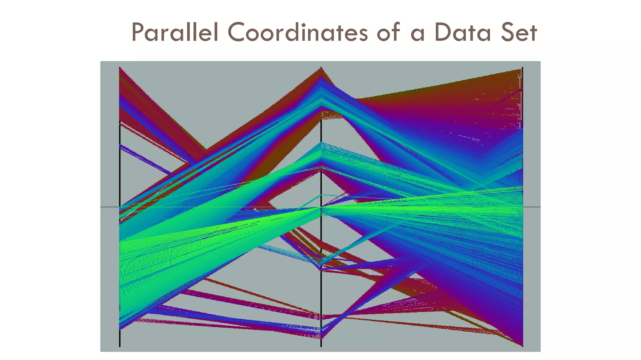
100. 101
Parallel Coordinates
 n equidistant axes which are parallel to
one of the screen axes and correspond
to the attributes
 The axes are scaled to the [minimum,
maximum]: range of the corresponding
attribute
 Every data item corresponds to a
polygonal line which intersects each of
the axes at the point which corresponds
to the value for the attribute

101. Parallel Coordinates of a Data Set

102. 103
Icon-Based Visualization Techniques
 Visualization of the data values as features of icons
 Typical visualization methods
 Chernoff Faces
 Stick Figures
 General techniques
 Shape coding: Use shape to represent certain information encoding
 Color icons: Use color icons to encode more information
 Tile bars: Use small icons to represent the relevant feature vectors in document
retrieval

103. 104
Chernoff Faces
 A way to display variables on a two-dimensional surface, e.g., let x be eyebrow slant,
y be eye size, z be nose length, etc.
 The figure shows faces produced using 10 characteristics--head eccentricity, eye size,
eye spacing, eye eccentricity, pupil size, eyebrow slant, nose size, mouth shape,
mouth size, and mouth opening): Each assigned one of 10 possible values, generated
using Mathematica (S. Dickson)
 REFERENCE: Gonick, L. and Smith, W. The
Cartoon Guide to Statistics. New York: Harper
Perennial, p. 212, 1993
 Weisstein, Eric W. "Chernoff Face." From
MathWorld--A Wolfram Web Resource.
mathworld.wolfram.com/ChernoffFace.html

104. Stick Figure
 A census data figure showing
age, income, gender,
education, etc.
 A 5-piece stick figure (1 body
and 4 limbs w. different
angle/length)

105. 106
Hierarchical Visualization Techniques
 Visualization of the data using a hierarchical partitioning into subspaces
 Methods
 Dimensional Stacking
 Worlds-within-Worlds
 Tree-Map
 Cone Trees
 InfoCube

106. 107
Dimensional Stacking
 Partitioning of the n-dimensional attribute space in 2-D subspaces, which are
‘stacked’ into each other
 Partitioning of the attribute value ranges into classes. The important attributes
should be used on the outer levels.
 Adequate for data with ordinal attributes of low cardinality
 But, difficult to display more than nine dimensions
 Important to map dimensions appropriately

107. Used by permission of M. Ward, Worcester Polytechnic Institute
Visualization of oil mining data with longitude and latitude mapped to the
outer x-, y-axes and ore grade and depth mapped to the inner x-, y-axes
Dimensional Stacking

108. 109
Worlds-within-Worlds
 Assign the function and two most important parameters to innermost world
 Fix all other parameters at constant values - draw other (1 or 2 or 3 dimensional
worlds choosing these as the axes)
 Software that uses this paradigm
 N–vision: Dynamic interaction through
data glove and stereo displays,
including rotation, scaling (inner) and
translation (inner/outer)
 Auto Visual: Static interaction by
means of queries

109. 110
Tree-Map
 Screen-filling method which uses a hierarchical partitioning of the screen into regions
depending on the attribute values
 The x- and y-dimension of the screen are partitioned alternately according to the
attribute values (classes)
Schneiderman@UMD: Tree-Map of a File System Schneiderman@UMD: Tree-Map to support
large data sets of a million items

110. 111
InfoCube
 A 3-D visualization technique where hierarchical information is displayed as nested
semi-transparent cubes
 The outermost cubes correspond to the top level data, while the subnodes or the lower
level data are represented as smaller cubes inside the outermost cubes, etc.

111. 112
Three-D Cone Trees
 3D cone tree visualization technique works well for
up to a thousand nodes or so
 First build a 2D circle tree that arranges its nodes in
concentric circles centered on the root node
 Cannot avoid overlaps when projected to 2D
 G. Robertson, J. Mackinlay, S. Card. “Cone Trees:
Animated 3D Visualizations of Hierarchical
Information”, ACM SIGCHI'91
 Graph from Nadeau Software Consulting website:
Visualize a social network data set that models the
way an infection spreads from one person to the next

112. 113
Visualizing Complex Data and Relations: Tag Cloud
 Tag cloud: Visualizing user-generated
tags
 The importance of tag is represented
by font size/color
 Popularly used to visualize
word/phrase distributions
Newsmap: Google News Stories in 2005
KDD 2013 Research Paper Title Tag Cloud

113. 114
Visualizing Complex Data and Relations: Social Networks
 Visualizing non-numerical data: social and information networks
A typical network structure A social network
organizing
information networks

114. 115
Standardizing Numeric Data
 Z-score:
 X: raw score to be standardized, μ: mean of the population, σ: standard deviation
 the distance between the raw score and the population mean in units of the standard deviation
 negative when the raw score is below the mean, positive when above
 An alternative way: Calculate the mean absolute deviation
where
 standardized measure (z-score):
 Using mean absolute deviation is more robust than using standard deviation
σ
µ
−
= x
z
.
)
...
2
1
1
nf
f
f
f
x
x
(x
n
m +
+
+
=
|)
|
...
|
|
|
(|
1
2
1 f
nf
f
f
f
f
f
m
x
m
x
m
x
n
s −
+
+
−
+
−
=
f
f
if
if s
m
x
z
−
=