Lect 2 getting to know your data

 Data Objects and Attribute Types
 Basic Statistical Descriptions of Data
 DataVisualization
 Measuring Data Similarity and Dissimilarity
 Summary

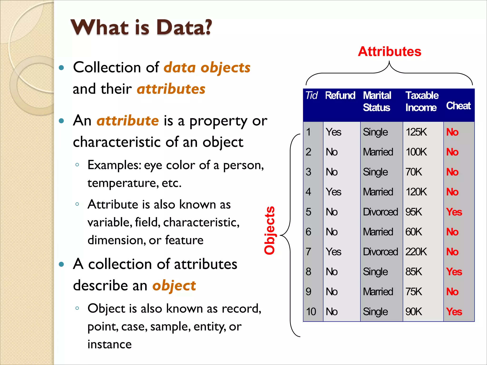
 Collection of data objects
and their attributes
 An attribute is a property or
characteristic of an object
◦ Examples: eye color of a person,
temperature, etc.
◦ Attribute is also known as
variable, field, characteristic,
dimension, or feature
 A collection of attributes
describe an object
◦ Object is also known as record,
point, case, sample, entity, or
instance
Tid Refund Marital
Status
Taxable
Income Cheat
1 Yes Single 125K No
2 No Married 100K No
3 No Single 70K No
4 Yes Married 120K No
5 No Divorced 95K Yes
6 No Married 60K No
7 Yes Divorced 220K No
8 No Single 85K Yes
9 No Married 75K No
10 No Single 90K Yes
10
Attributes
Objects

 Dimensionality
◦ Curse of dimensionality
 Sparsity
◦ Only presence counts
 Resolution
◦ Patterns depend on the scale
 Distribution
◦ Centrality and dispersion

 Data may have parts
 The different parts of the data may have
relationships
 More generally, data may have structure
 Data can be incomplete
We will discuss this in more detail later........

 Data sets are made up of data objects.
 A data object represents an entity.
 Examples:
◦ sales database: customers, store items, sales
◦ medical database: patients, treatments
◦ university database: students, professors, courses
 Also called samples , examples, instances, data points,
objects, tuples.
 Data objects are described by attributes.
 Database rows -> data objects; columns ->attributes.

 Attribute (or dimensions, features, variables):
A data field, representing a characteristic or feature of
a data object.
◦ E.g., customer _ID, name, address
• Observed values for a given attribute are known as
observations.
• A set of attributes used to describe a given object is
called an attribute vector (or feature vector ).
• The distribution of data involving one attribute (or
variable) is called univariate.
• A bivariate distribution involves two attributes, and so
on.

 Attribute values are numbers or symbols
assigned to an attribute for a particular object
 Distinction between attributes and attribute
values
◦ Same attribute can be mapped to different attribute
values
 Example: height can be measured in feet or meters
◦ Different attributes can be mapped to the same set of
values
 Example:Attribute values for ID and age are integers
 But properties of attribute values can be different

9
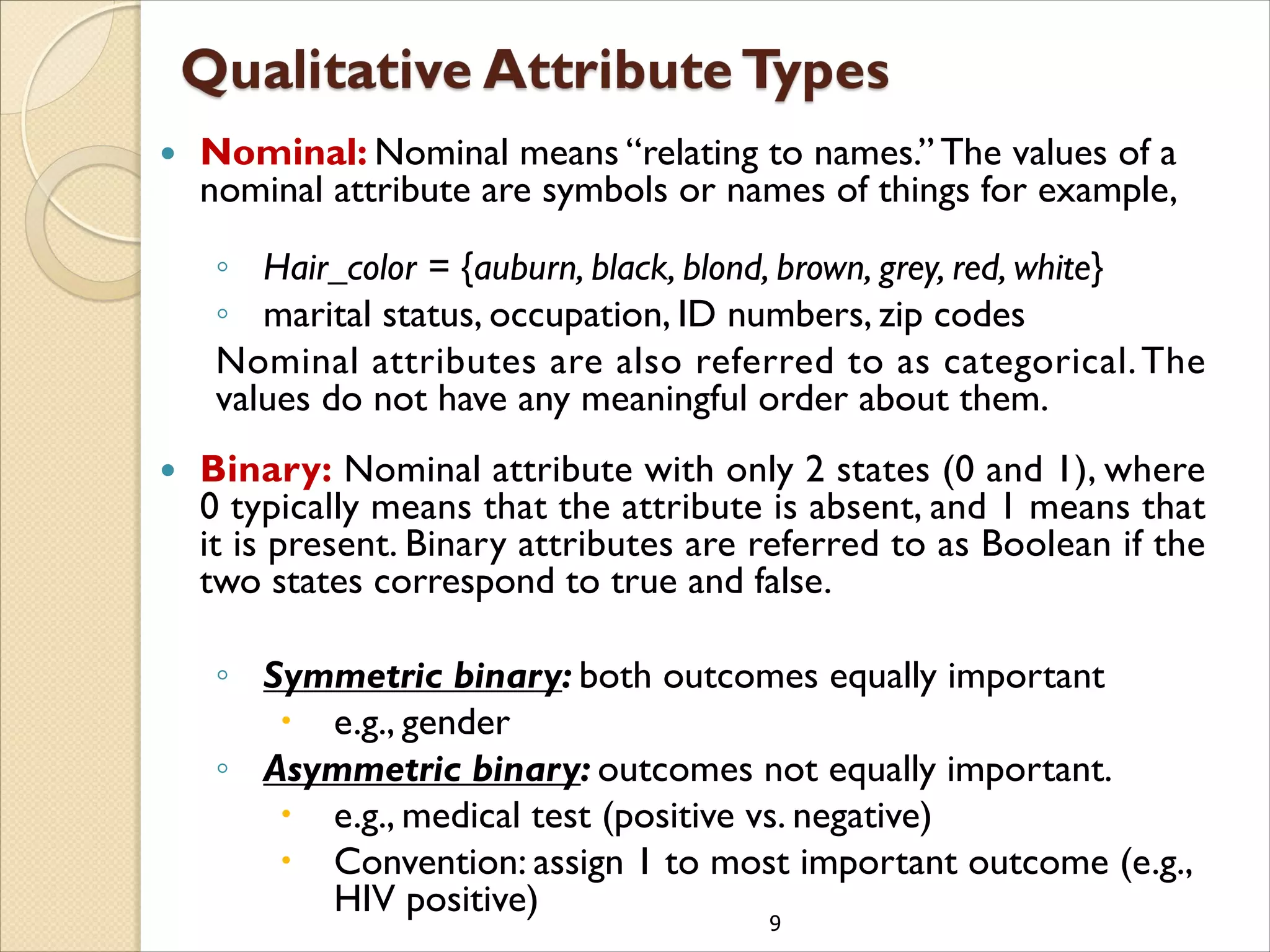
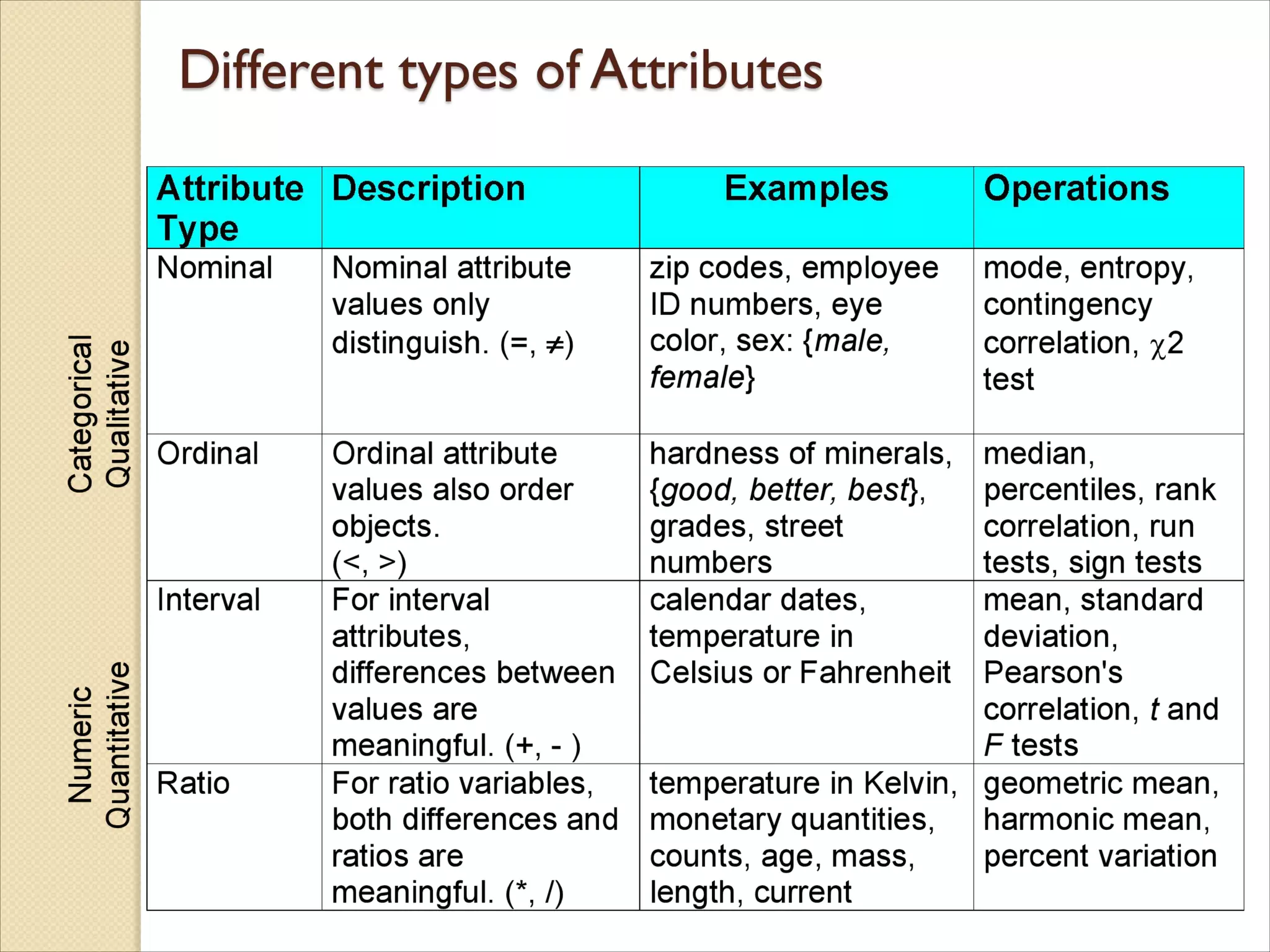
 Nominal: Nominal means “relating to names.” The values of a
nominal attribute are symbols or names of things for example,
◦ Hair_color = {auburn, black, blond, brown, grey, red, white}
◦ marital status, occupation, ID numbers, zip codes
Nominal attributes are also referred to as categorical.The
values do not have any meaningful order about them.
 Binary: Nominal attribute with only 2 states (0 and 1), where
0 typically means that the attribute is absent, and 1 means that
it is present. Binary attributes are referred to as Boolean if the
two states correspond to true and false.
◦ Symmetric binary: both outcomes equally important
 e.g., gender
◦ Asymmetric binary: outcomes not equally important.
 e.g., medical test (positive vs. negative)
 Convention: assign 1 to most important outcome (e.g.,
HIV positive)

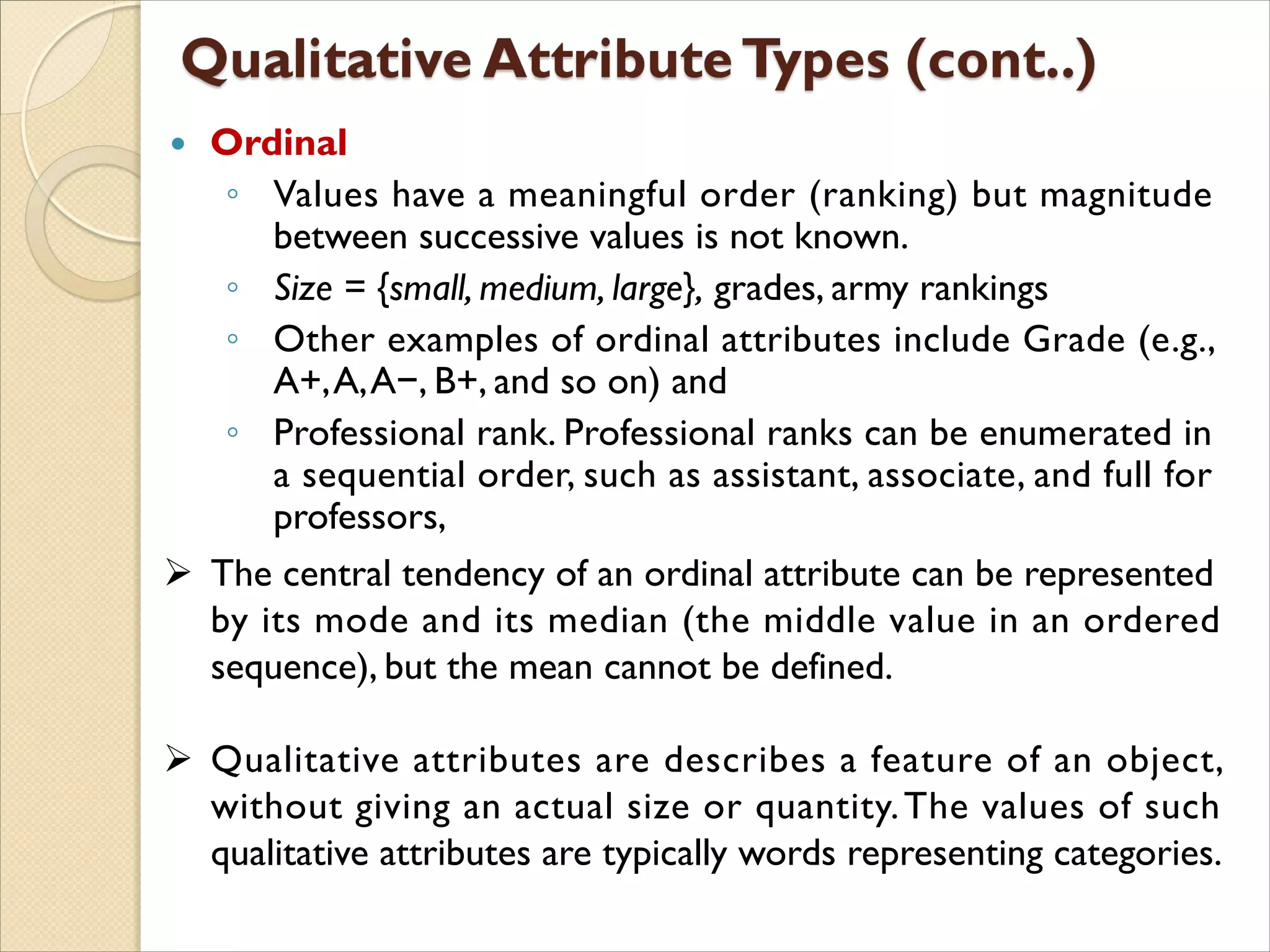
 Ordinal
◦ Values have a meaningful order (ranking) but magnitude
between successive values is not known.
◦ Size = {small, medium, large}, grades, army rankings
◦ Other examples of ordinal attributes include Grade (e.g.,
A+,A,A−, B+, and so on) and
◦ Professional rank. Professional ranks can be enumerated in
a sequential order, such as assistant, associate, and full for
professors,
 The central tendency of an ordinal attribute can be represented
by its mode and its median (the middle value in an ordered
sequence), but the mean cannot be defined.
 Qualitative attributes are describes a feature of an object,
without giving an actual size or quantity.The values of such
qualitative attributes are typically words representing categories.

11
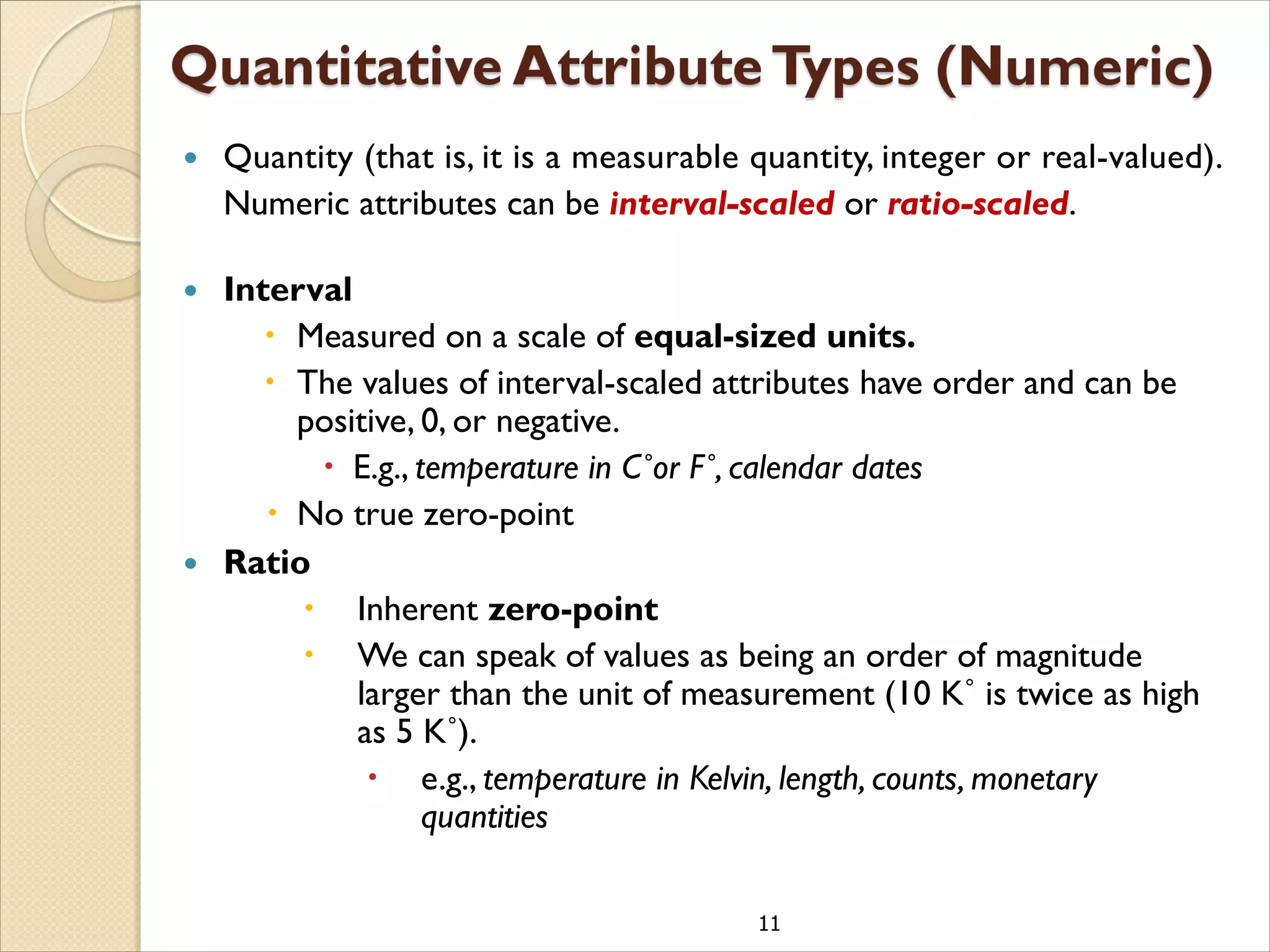
 Quantity (that is, it is a measurable quantity, integer or real-valued).
Numeric attributes can be interval-scaled or ratio-scaled.
 Interval
 Measured on a scale of equal-sized units.
 The values of interval-scaled attributes have order and can be
positive, 0, or negative.
 E.g., temperature in C˚or F˚, calendar dates
 No true zero-point
 Ratio
 Inherent zero-point
 We can speak of values as being an order of magnitude
larger than the unit of measurement (10 K˚ is twice as high
as 5 K˚).
 e.g., temperature in Kelvin, length, counts, monetary
quantities

12
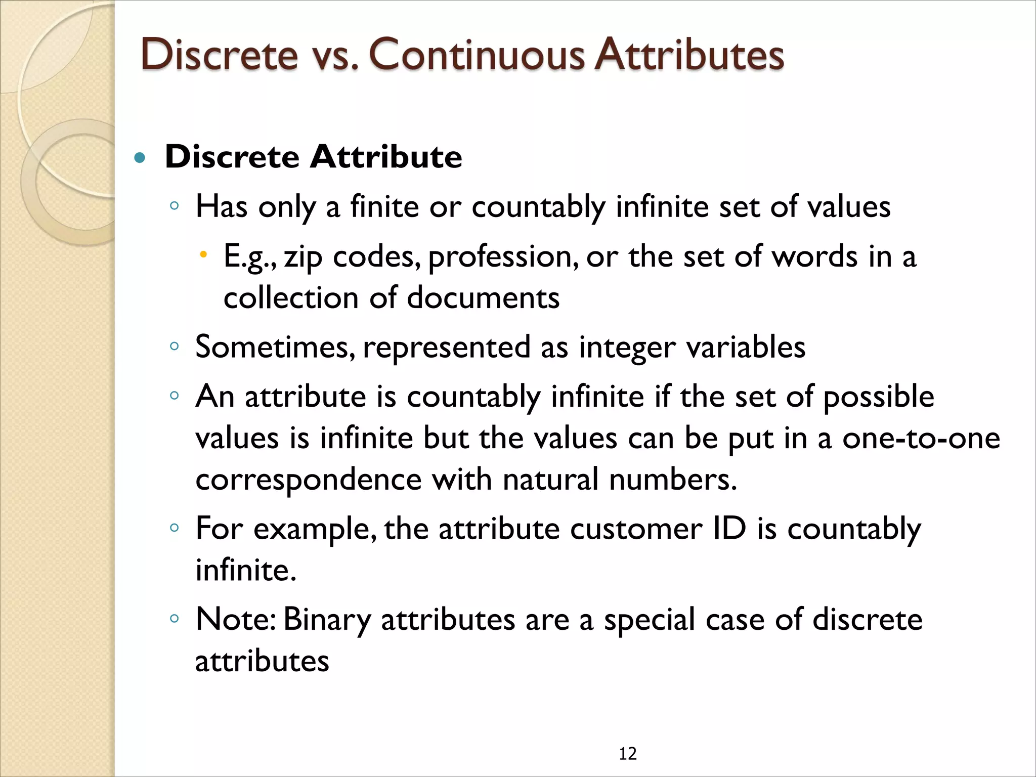
 Discrete Attribute
◦ Has only a finite or countably infinite set of values
 E.g., zip codes, profession, or the set of words in a
collection of documents
◦ Sometimes, represented as integer variables
◦ An attribute is countably infinite if the set of possible
values is infinite but the values can be put in a one-to-one
correspondence with natural numbers.
◦ For example, the attribute customer ID is countably
infinite.
◦ Note: Binary attributes are a special case of discrete
attributes

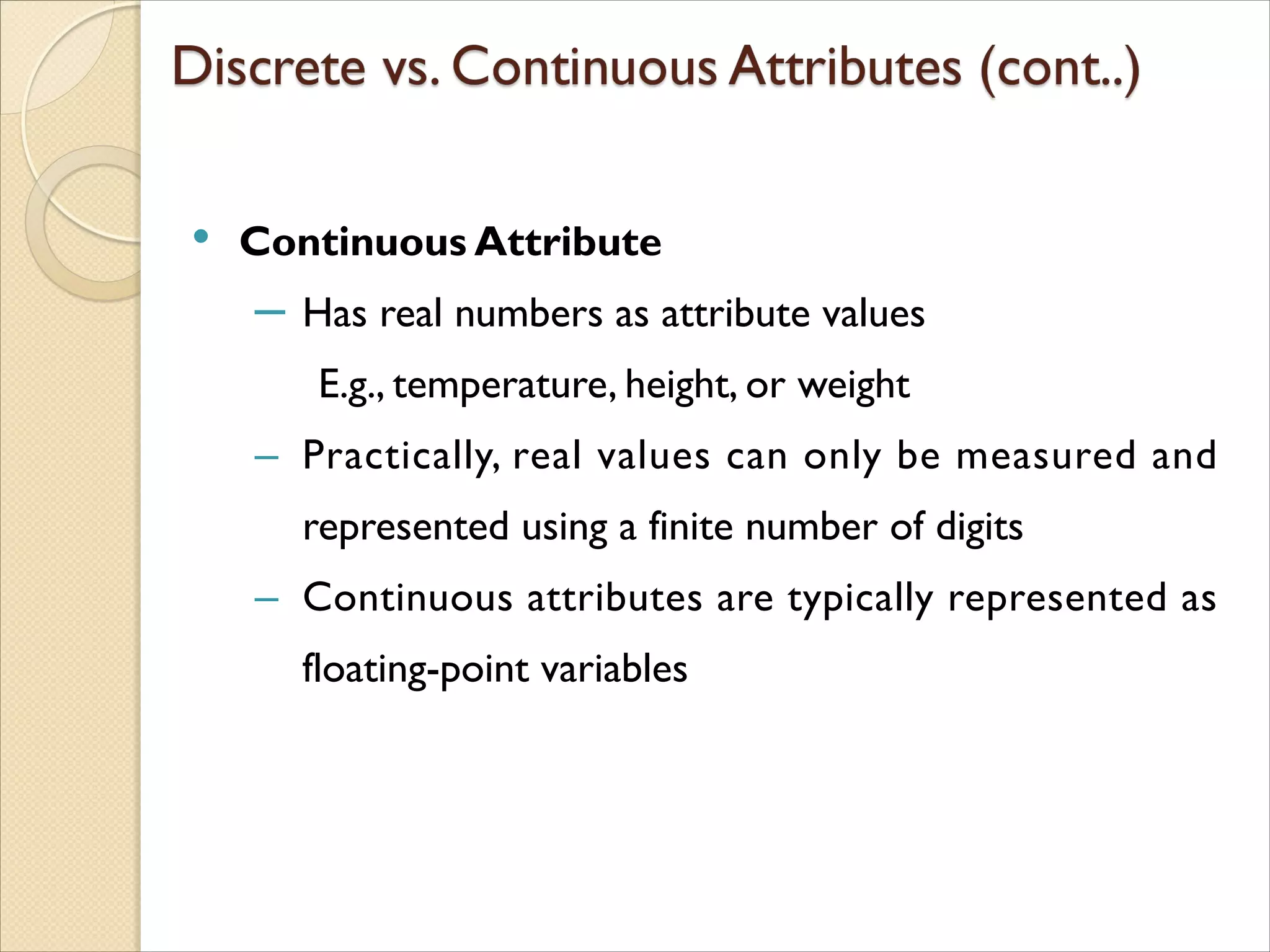
• Continuous Attribute
‒ Has real numbers as attribute values
E.g., temperature, height, or weight
‒ Practically, real values can only be measured and
represented using a finite number of digits
‒ Continuous attributes are typically represented as
floating-point variables

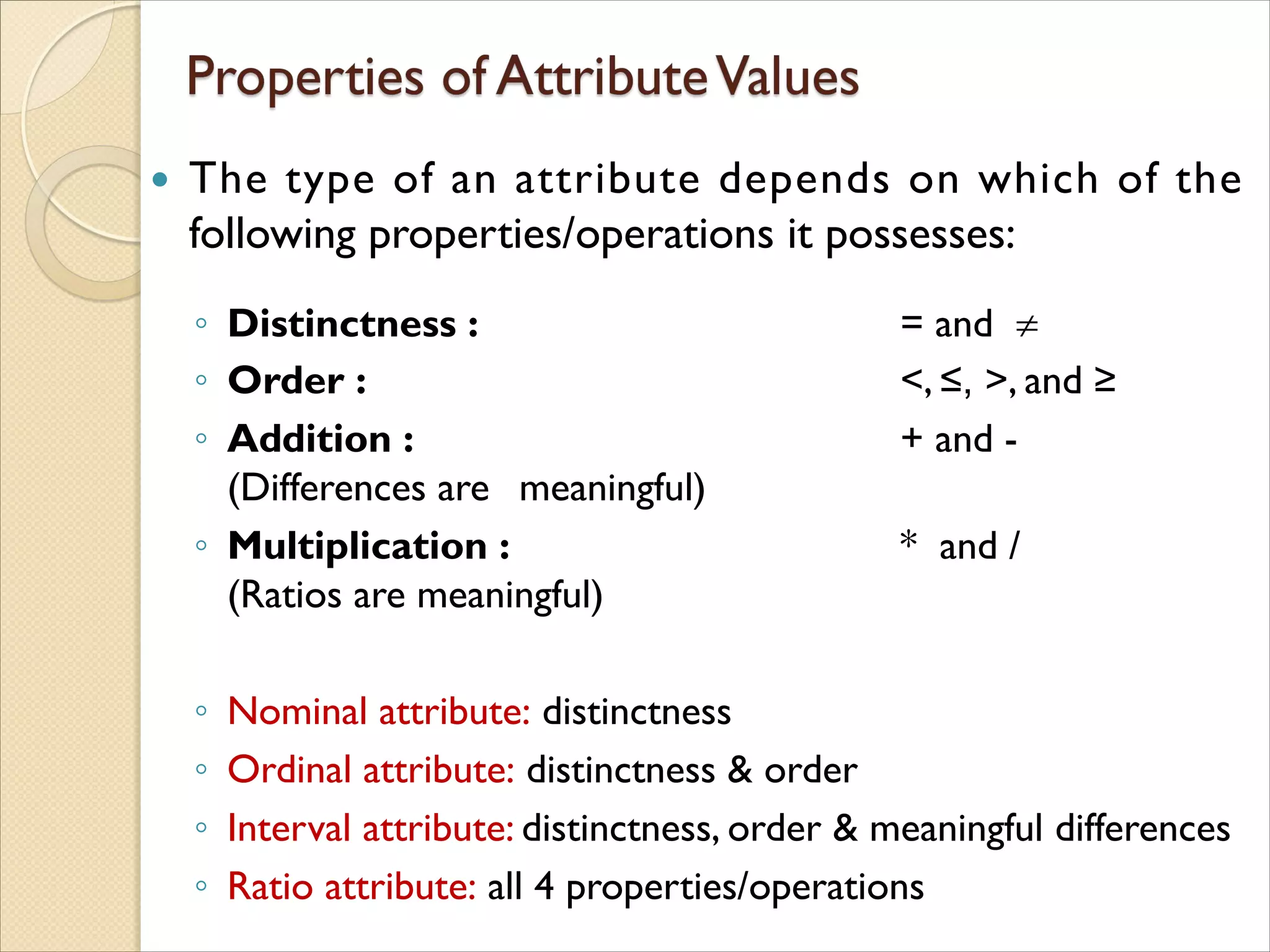
 The type of an attribute depends on which of the
following properties/operations it possesses:
◦ Distinctness : = and 
◦ Order : <, ≤, >, and ≥
◦ Addition : + and -
(Differences are meaningful)
◦ Multiplication : * and /
(Ratios are meaningful)
◦ Nominal attribute: distinctness
◦ Ordinal attribute: distinctness & order
◦ Interval attribute: distinctness, order & meaningful differences
◦ Ratio attribute: all 4 properties/operations

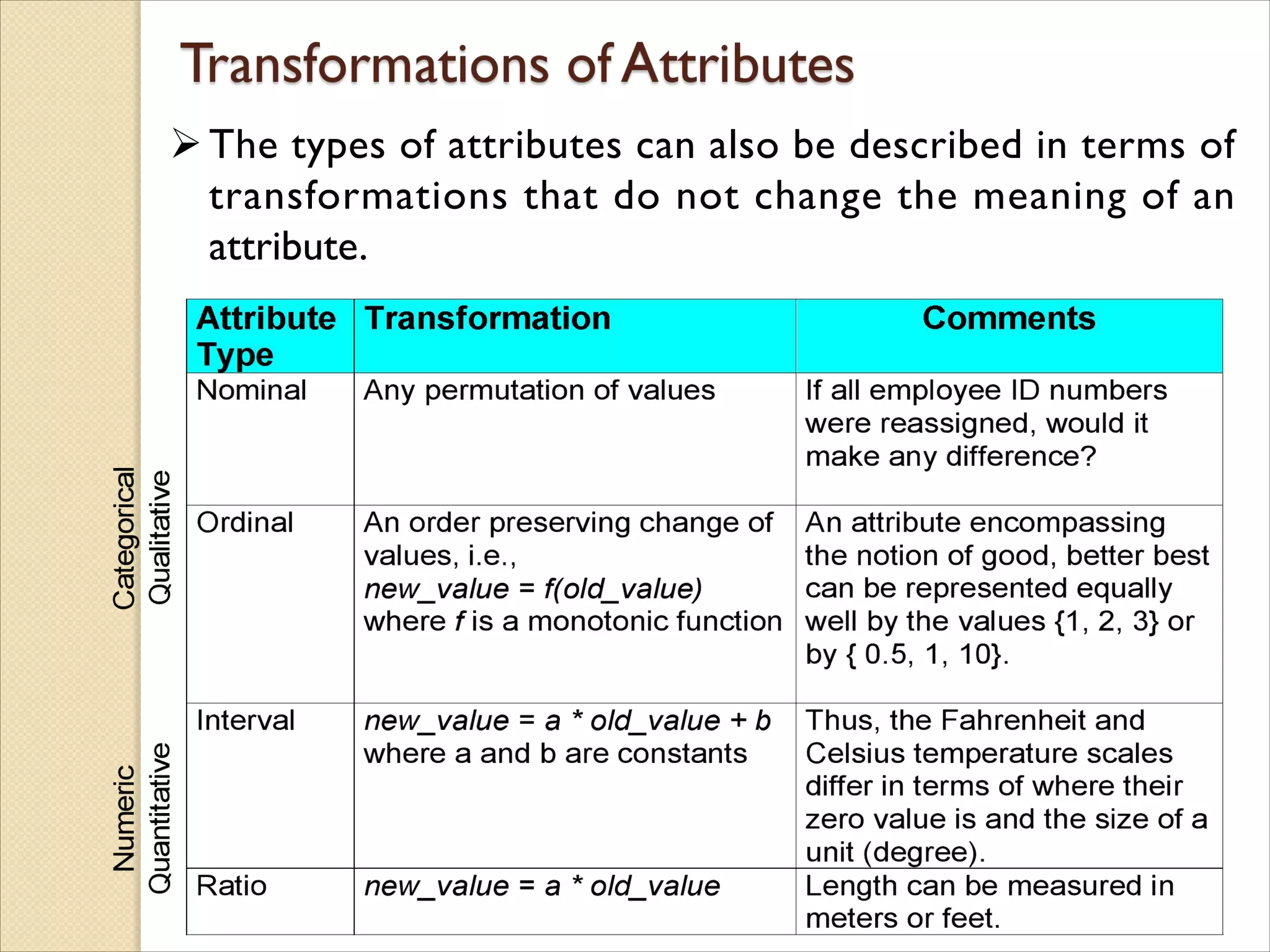
The types of attributes can also be described in terms of
transformations that do not change the meaning of an
attribute.

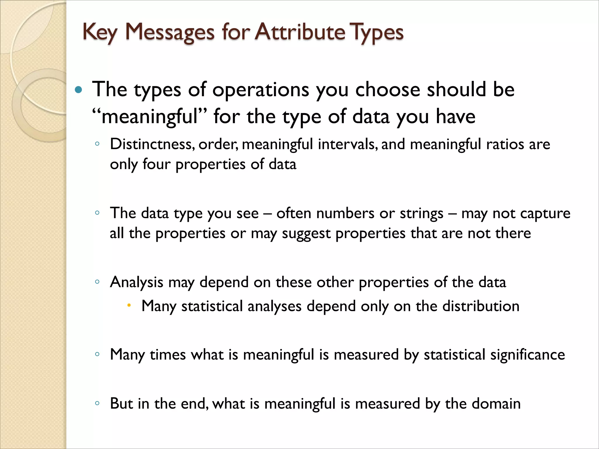
 The types of operations you choose should be
“meaningful” for the type of data you have
◦ Distinctness, order, meaningful intervals, and meaningful ratios are
only four properties of data
◦ The data type you see – often numbers or strings – may not capture
all the properties or may suggest properties that are not there
◦ Analysis may depend on these other properties of the data
 Many statistical analyses depend only on the distribution
◦ Many times what is meaningful is measured by statistical significance
◦ But in the end, what is meaningful is measured by the domain

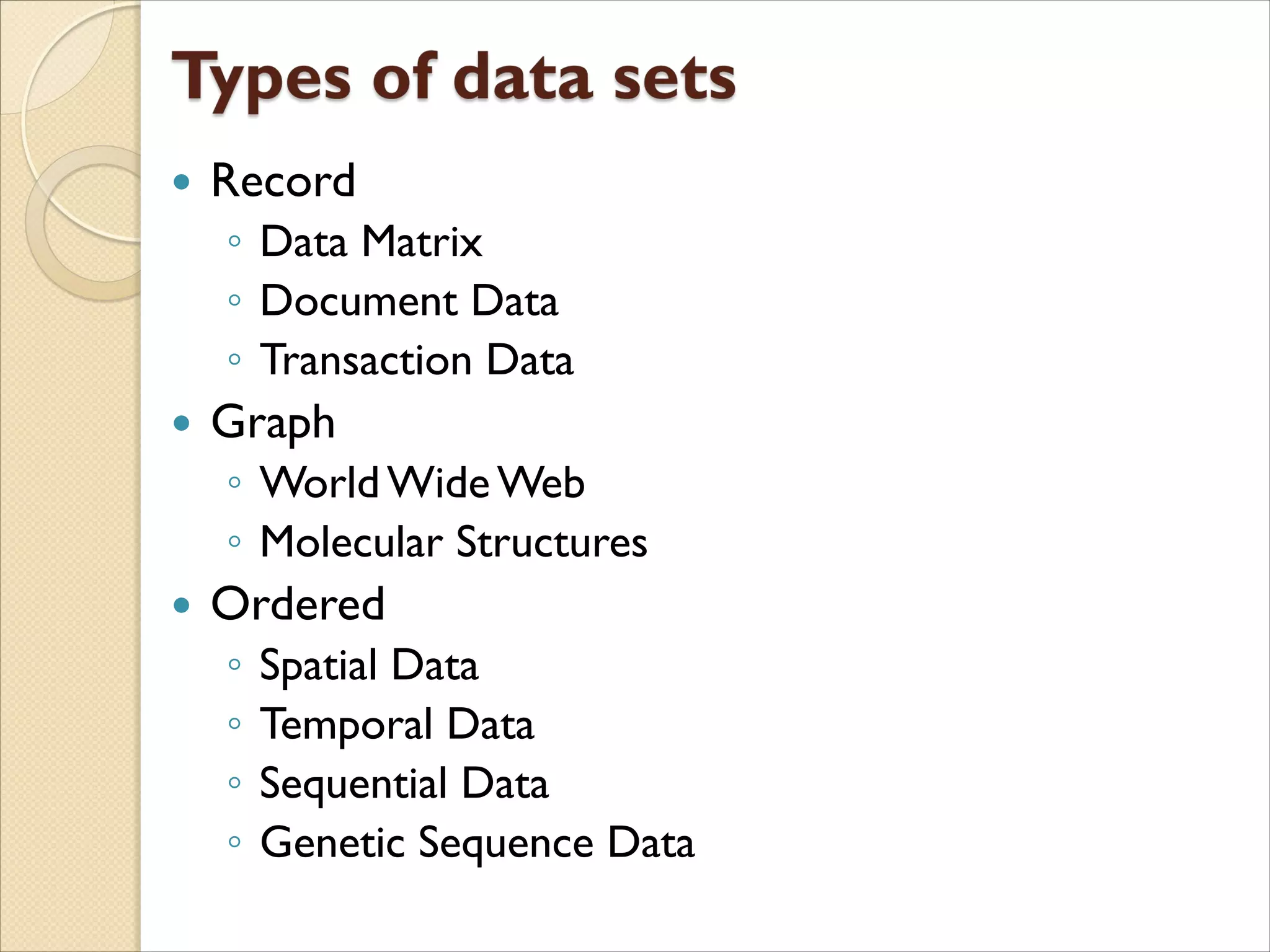
 Record
◦ Data Matrix
◦ Document Data
◦ Transaction Data
 Graph
◦ World Wide Web
◦ Molecular Structures
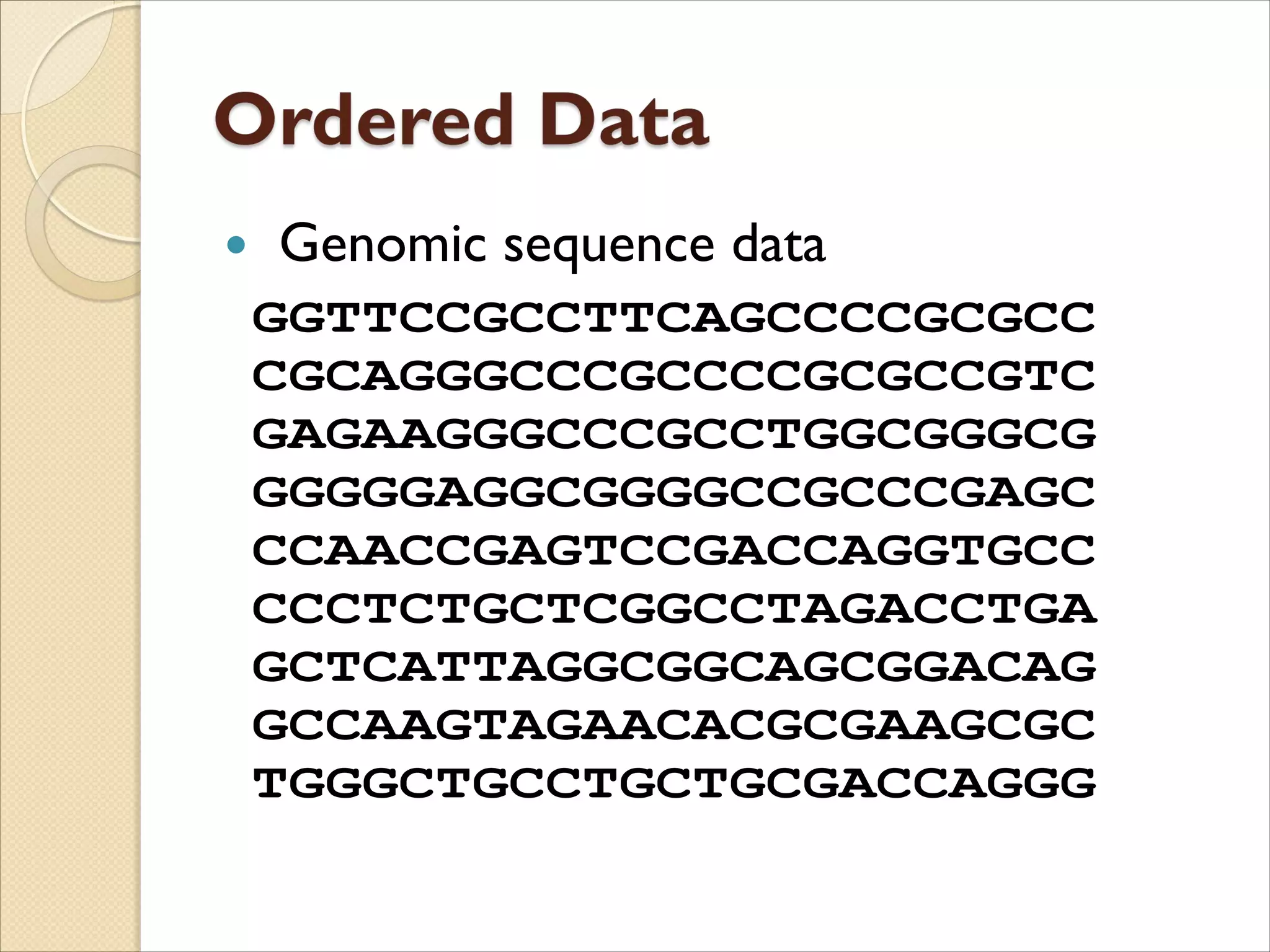
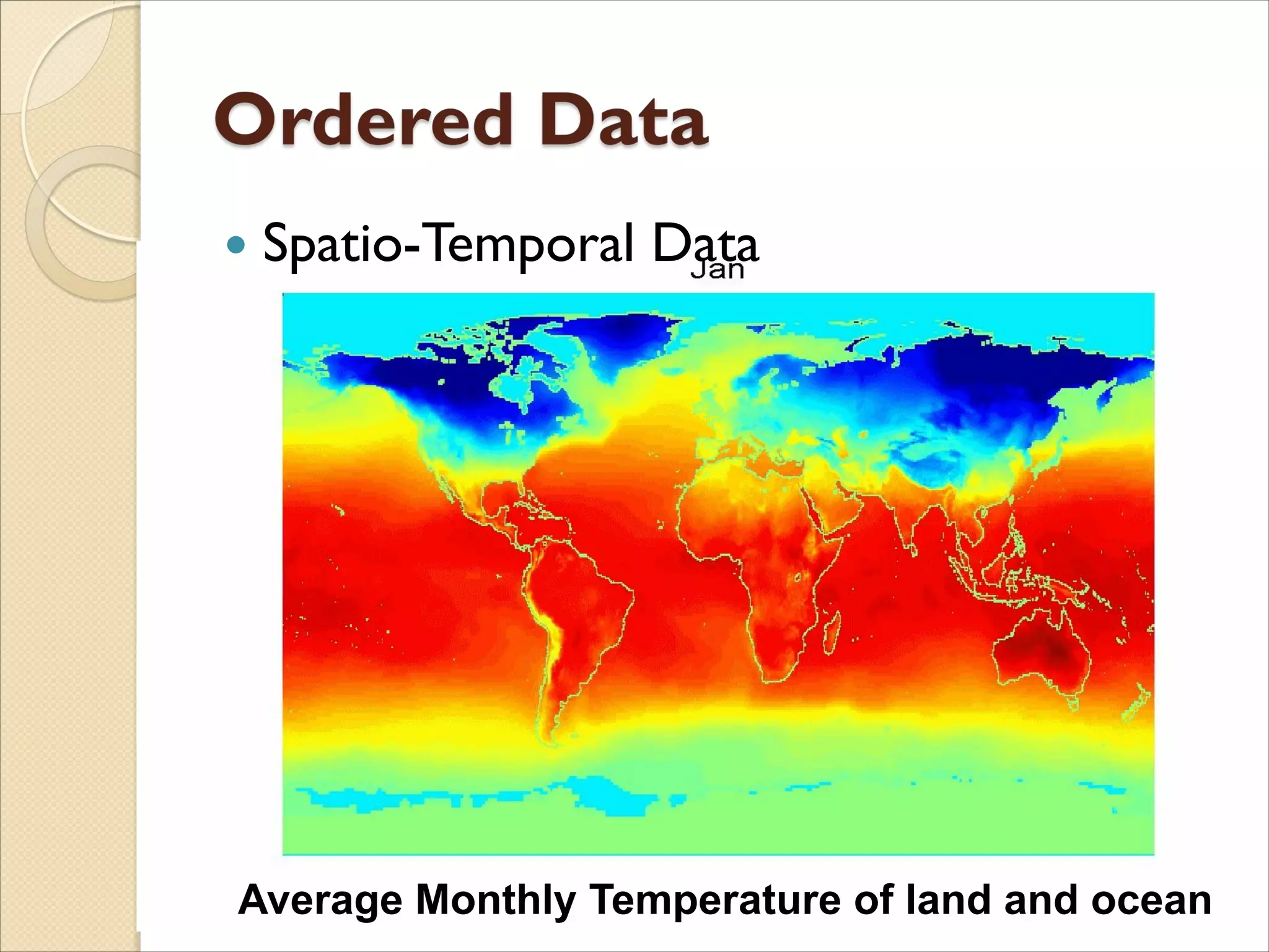
 Ordered
◦ Spatial Data
◦ Temporal Data
◦ Sequential Data
◦ Genetic Sequence Data

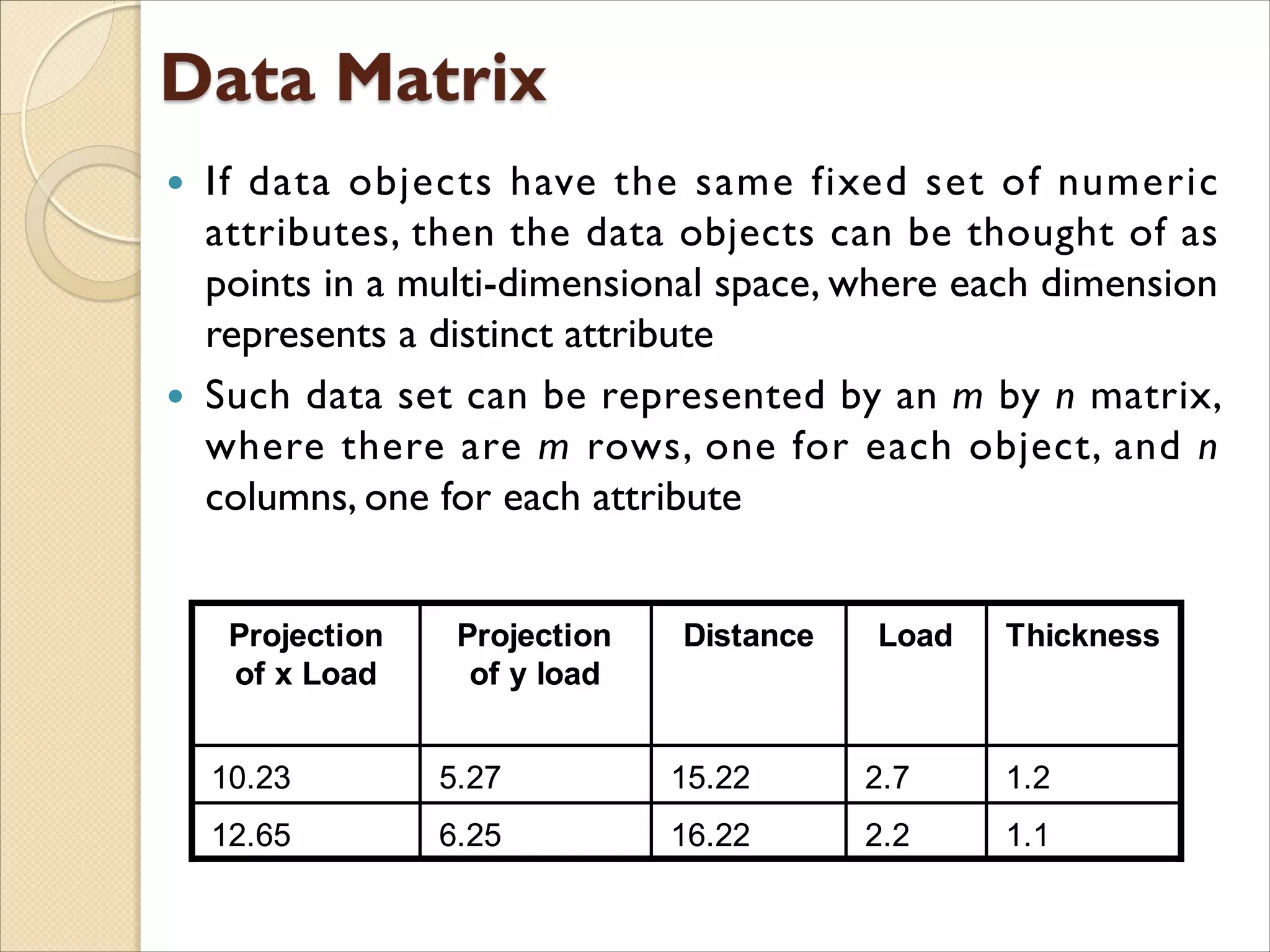
 If data objects have the same fixed set of numeric
attributes, then the data objects can be thought of as
points in a multi-dimensional space, where each dimension
represents a distinct attribute
 Such data set can be represented by an m by n matrix,
where there are m rows, one for each object, and n
columns, one for each attribute
1.12.216.226.2512.65
1.22.715.225.2710.23
ThicknessLoadDistanceProjection
of y load
Projection
of x Load
1.12.216.226.2512.65
1.22.715.225.2710.23
ThicknessLoadDistanceProjection
of y load
Projection
of x Load

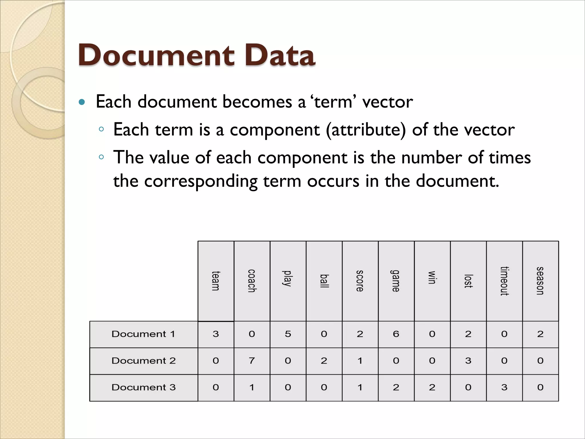
 Each document becomes a ‘term’ vector
◦ Each term is a component (attribute) of the vector
◦ The value of each component is the number of times
the corresponding term occurs in the document.

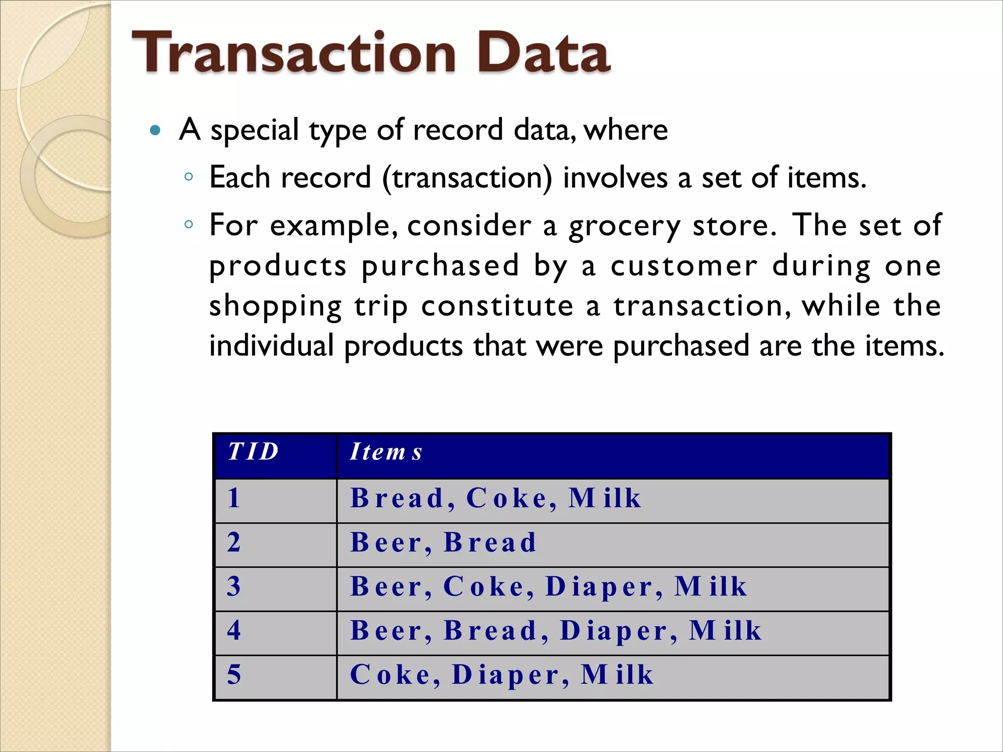
 A special type of record data, where
◦ Each record (transaction) involves a set of items.
◦ For example, consider a grocery store. The set of
products purchased by a customer during one
shopping trip constitute a transaction, while the
individual products that were purchased are the items.
T ID Item s
1 B read, C oke, M ilk
2 B eer, B read
3 B eer, C oke, D iap er, M ilk
4 B eer, B read , D iap er, M ilk
5 C oke, D iaper, M ilk

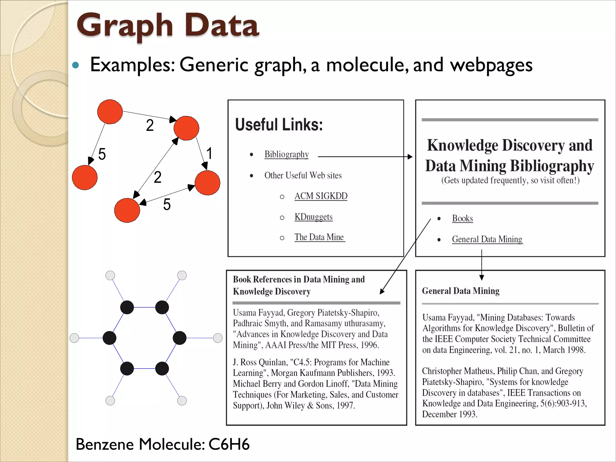
 Examples: Generic graph, a molecule, and webpages
5
2
1
2
5
Benzene Molecule: C6H6

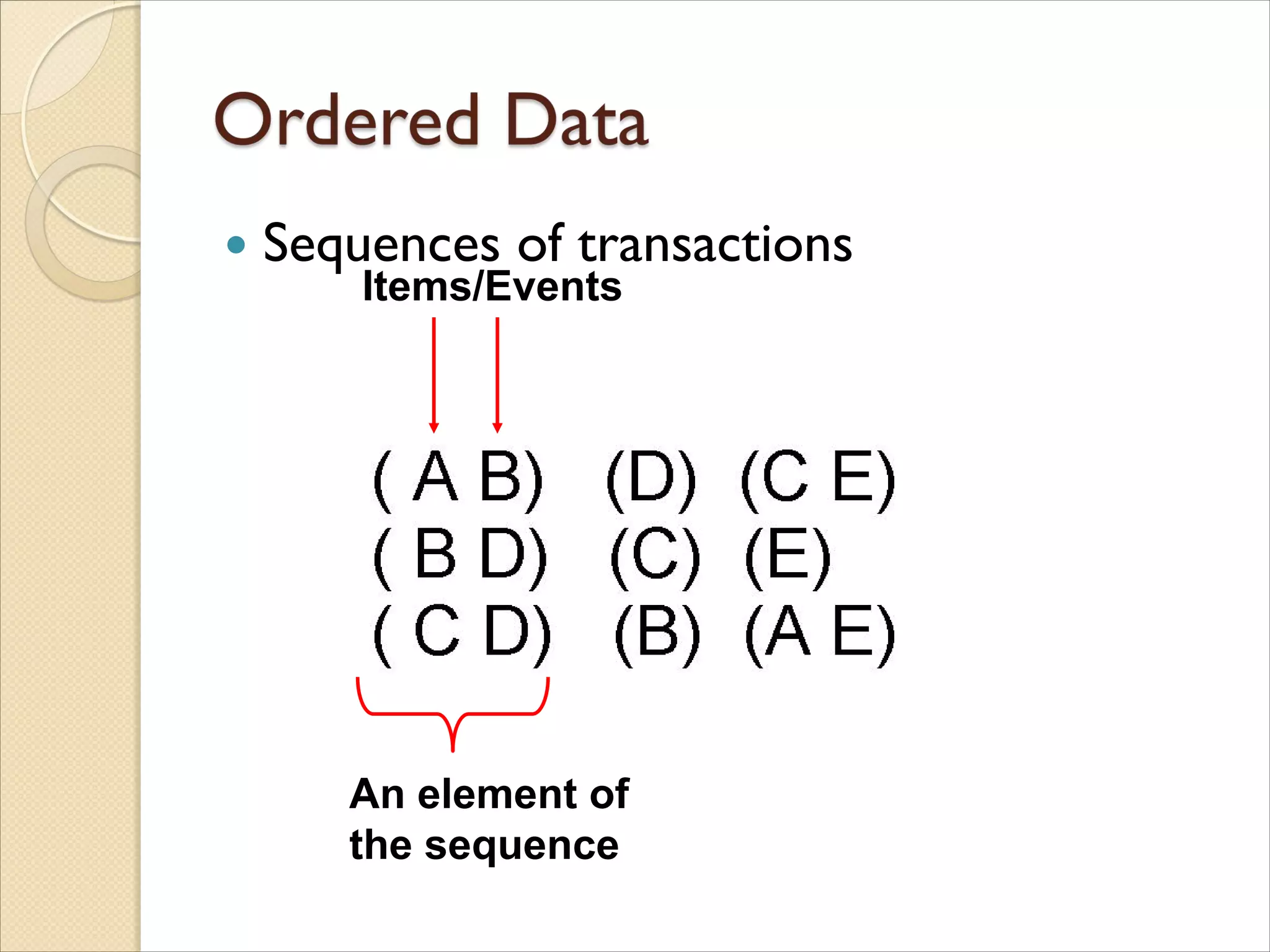
 Sequences of transactions
An element of
the sequence
Items/Events

 Genomic sequence data
GGTTCCGCCTTCAGCCCCGCGCC
CGCAGGGCCCGCCCCGCGCCGTC
GAGAAGGGCCCGCCTGGCGGGCG
GGGGGAGGCGGGGCCGCCCGAGC
CCAACCGAGTCCGACCAGGTGCC
CCCTCTGCTCGGCCTAGACCTGA
GCTCATTAGGCGGCAGCGGACAG
GCCAAGTAGAACACGCGAAGCGC
TGGGCTGCCTGCTGCGACCAGGG

 Spatio-Temporal Data
Average Monthly Temperature of land and ocean

 What kinds of data quality problems?
 How can we detect problems with the data?
 What can we do about these problems?
 Examples of data quality problems:
◦ Noise and outliers
◦ Missing values
◦ Duplicate data
◦ Wrong data

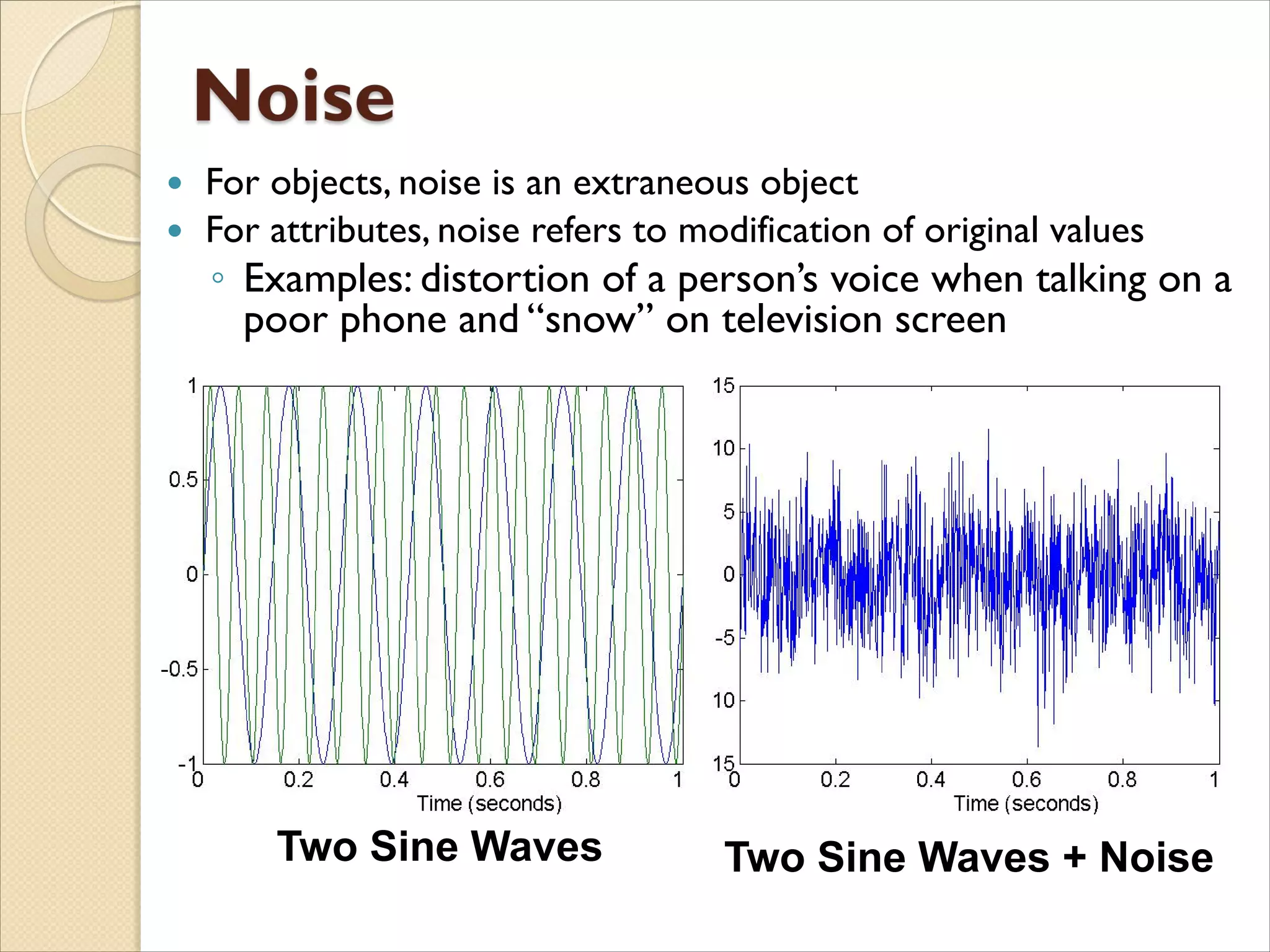
 For objects, noise is an extraneous object
 For attributes, noise refers to modification of original values
◦ Examples: distortion of a person’s voice when talking on a
poor phone and “snow” on television screen
Two Sine Waves Two Sine Waves + Noise

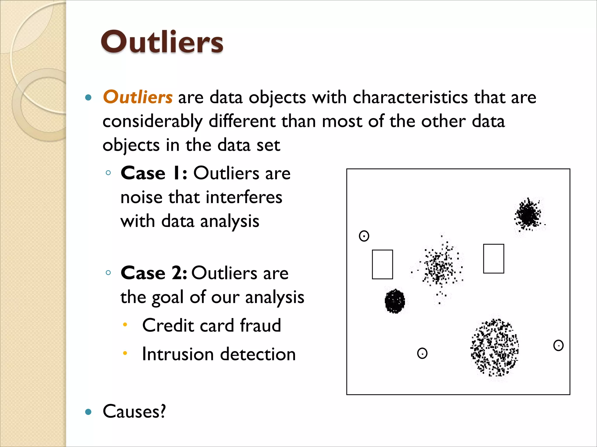
 Outliers are data objects with characteristics that are
considerably different than most of the other data
objects in the data set
◦ Case 1: Outliers are
noise that interferes
with data analysis
◦ Case 2: Outliers are
the goal of our analysis
 Credit card fraud
 Intrusion detection
 Causes?

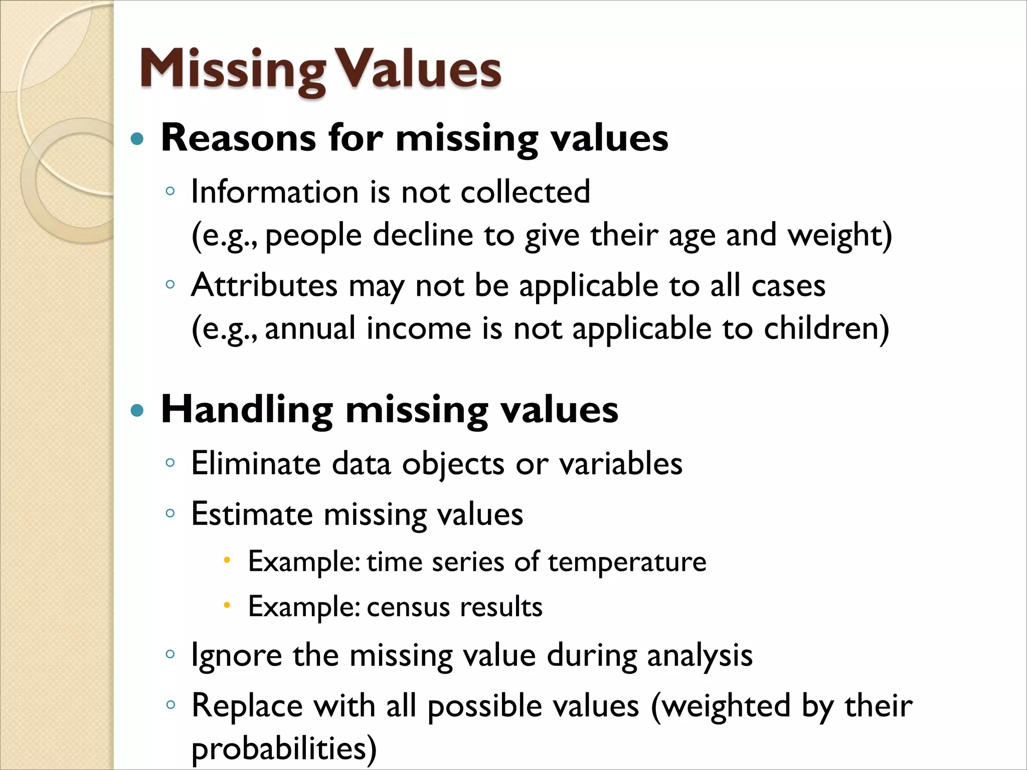
 Reasons for missing values
◦ Information is not collected
(e.g., people decline to give their age and weight)
◦ Attributes may not be applicable to all cases
(e.g., annual income is not applicable to children)
 Handling missing values
◦ Eliminate data objects or variables
◦ Estimate missing values
 Example: time series of temperature
 Example: census results
◦ Ignore the missing value during analysis
◦ Replace with all possible values (weighted by their
probabilities)

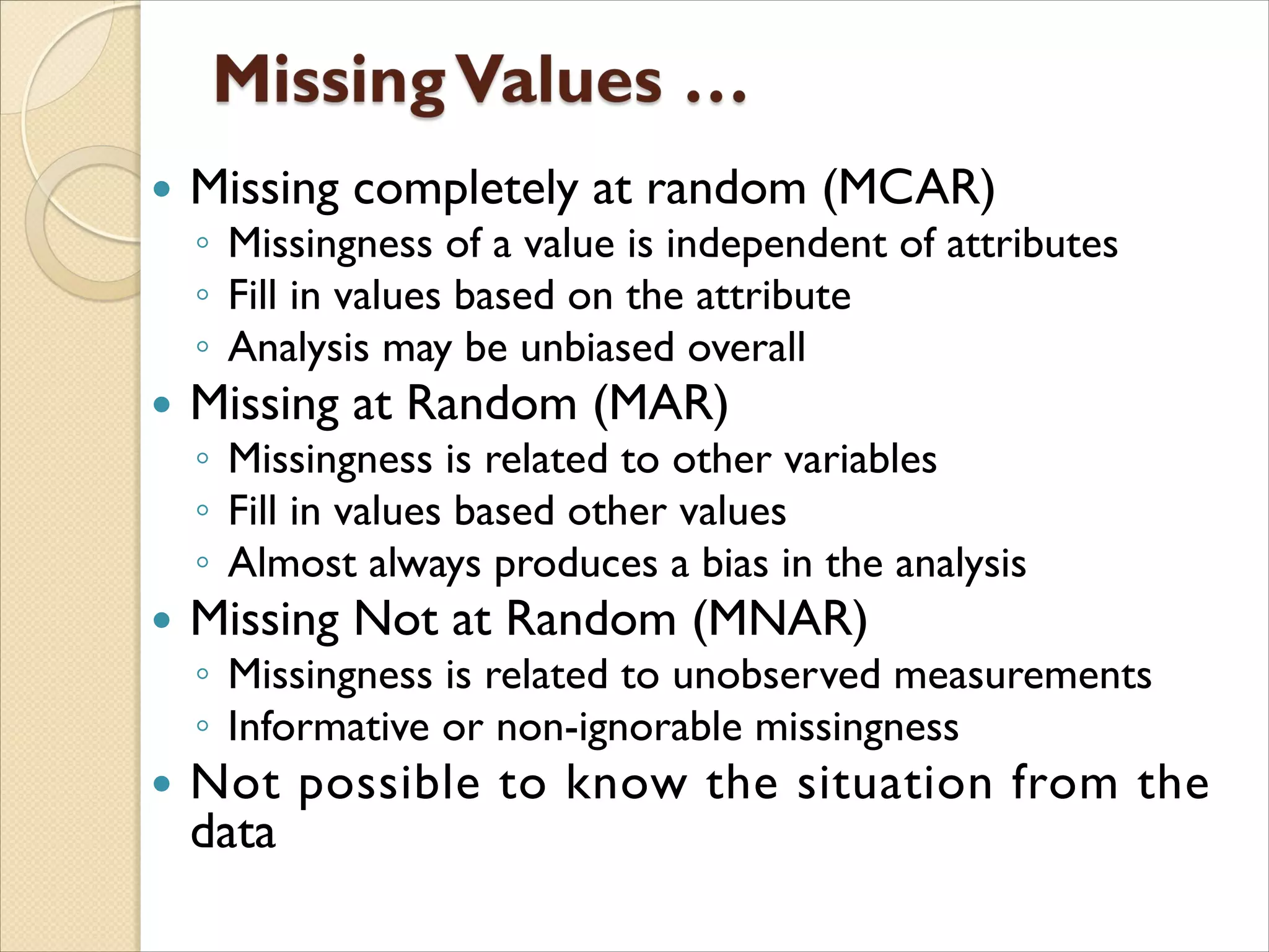
 Missing completely at random (MCAR)
◦ Missingness of a value is independent of attributes
◦ Fill in values based on the attribute
◦ Analysis may be unbiased overall
 Missing at Random (MAR)
◦ Missingness is related to other variables
◦ Fill in values based other values
◦ Almost always produces a bias in the analysis
 Missing Not at Random (MNAR)
◦ Missingness is related to unobserved measurements
◦ Informative or non-ignorable missingness
 Not possible to know the situation from the
data

 Data set may include data objects that are
duplicates, or almost duplicates of one another
◦ Major issue when merging data from heterogeneous
sources
 Examples:
◦ Same person with multiple email addresses
 Data cleaning
◦ Process of dealing with duplicate data issues
 When should duplicate data not be removed?

 Similarity measure
◦ Numerical measure of how alike two data objects are.
◦ Is higher when objects are more alike.
◦ Often falls in the range [0,1]
 Dissimilarity measure
◦ Numerical measure of how different two data objects
are
◦ Lower when objects are more alike
◦ Minimum dissimilarity is often 0
◦ Upper limit varies
 Proximity refers to a similarity or dissimilarity

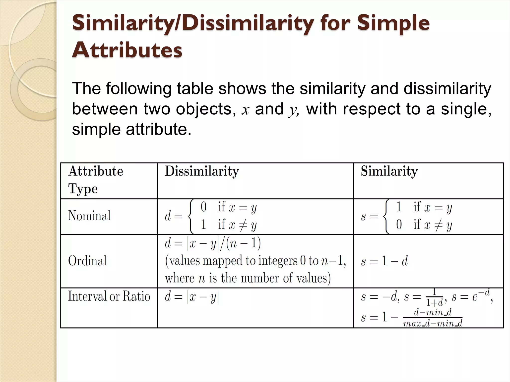
The following table shows the similarity and dissimilarity
between two objects, x and y, with respect to a single,
simple attribute.

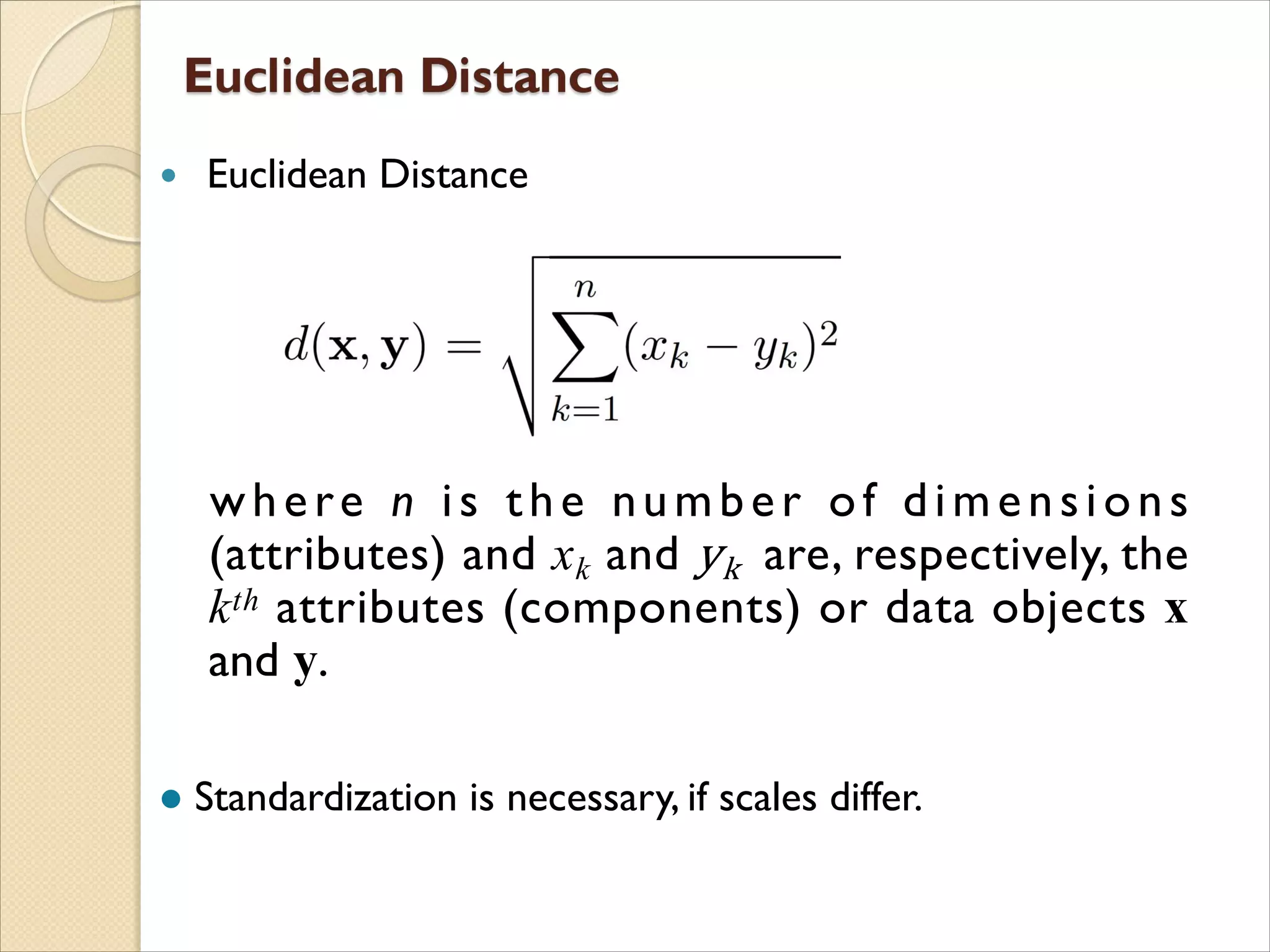
 Euclidean Distance
where n is the number of dimensions
(attributes) and xk and yk are, respectively, the
kth attributes (components) or data objects x
and y.
l Standardization is necessary, if scales differ.

0
1
2
3
0 1 2 3 4 5 6
p1
p2
p3 p4
point x y
p1 0 2
p2 2 0
p3 3 1
p4 5 1
Distance Matrix
p1 p2 p3 p4
p1 0 2.828 3.162 5.099
p2 2.828 0 1.414 3.162
p3 3.162 1.414 0 2
p4 5.099 3.162 2 0

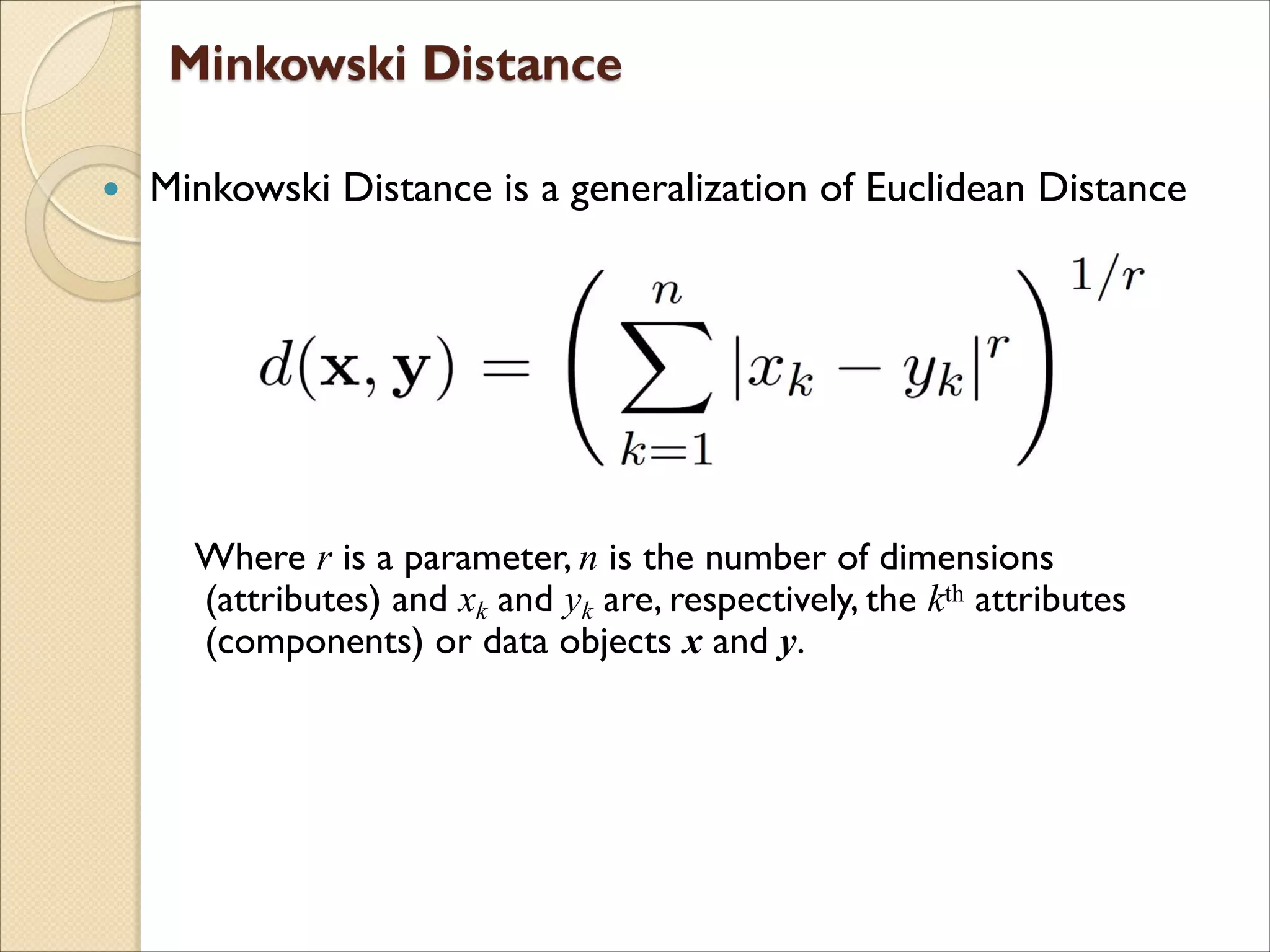
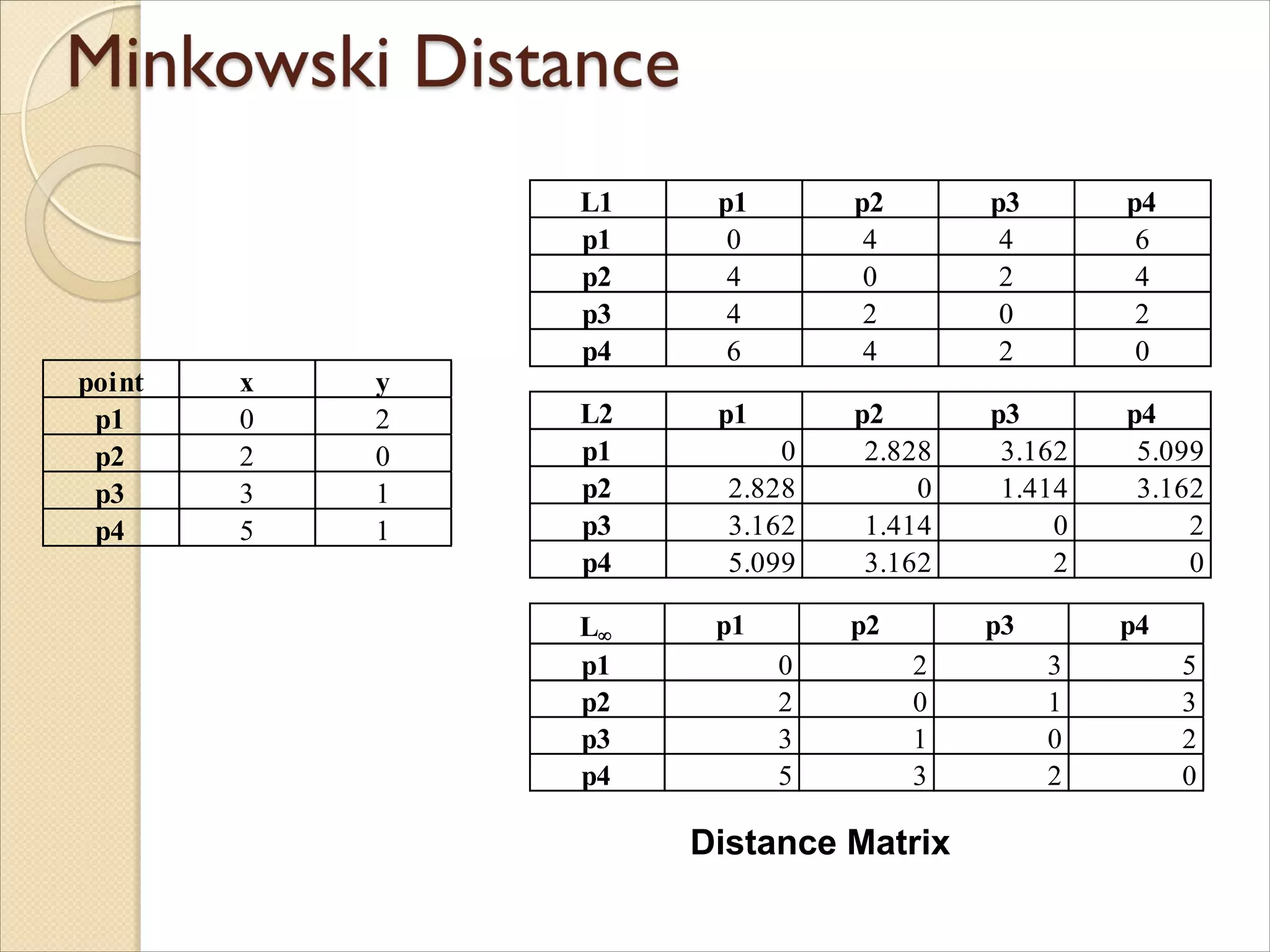
 Minkowski Distance is a generalization of Euclidean Distance
Where r is a parameter, n is the number of dimensions
(attributes) and xk and yk are, respectively, the kth attributes
(components) or data objects x and y.

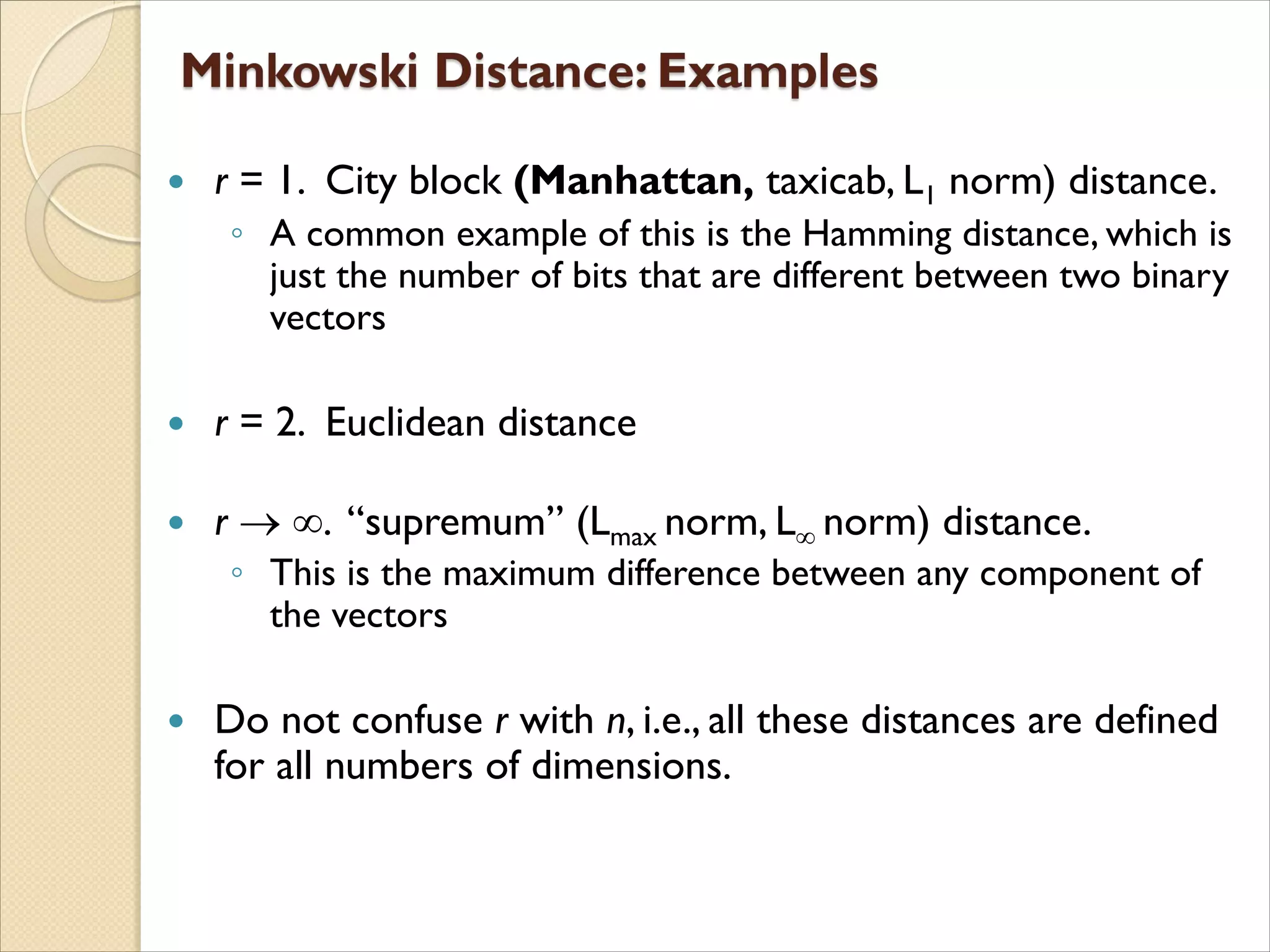
 r = 1. City block (Manhattan, taxicab, L1 norm) distance.
◦ A common example of this is the Hamming distance, which is
just the number of bits that are different between two binary
vectors
 r = 2. Euclidean distance
 r  . “supremum” (Lmax norm, L norm) distance.
◦ This is the maximum difference between any component of
the vectors
 Do not confuse r with n, i.e., all these distances are defined
for all numbers of dimensions.

Distance Matrix
point x y
p1 0 2
p2 2 0
p3 3 1
p4 5 1
L1 p1 p2 p3 p4
p1 0 4 4 6
p2 4 0 2 4
p3 4 2 0 2
p4 6 4 2 0
L2 p1 p2 p3 p4
p1 0 2.828 3.162 5.099
p2 2.828 0 1.414 3.162
p3 3.162 1.414 0 2
p4 5.099 3.162 2 0
L p1 p2 p3 p4
p1 0 2 3 5
p2 2 0 1 3
p3 3 1 0 2
p4 5 3 2 0

For red points, the Euclidean distance is 14.7, Mahalanobis distance is 6.
 is the covariance matrix

Covariance
Matrix:







3.02.0
2.03.0
A: (0.5, 0.5)
B: (0, 1)
C: (1.5, 1.5)
Mahal(A,B) = 5
Mahal(A,C) = 4
B
A
C

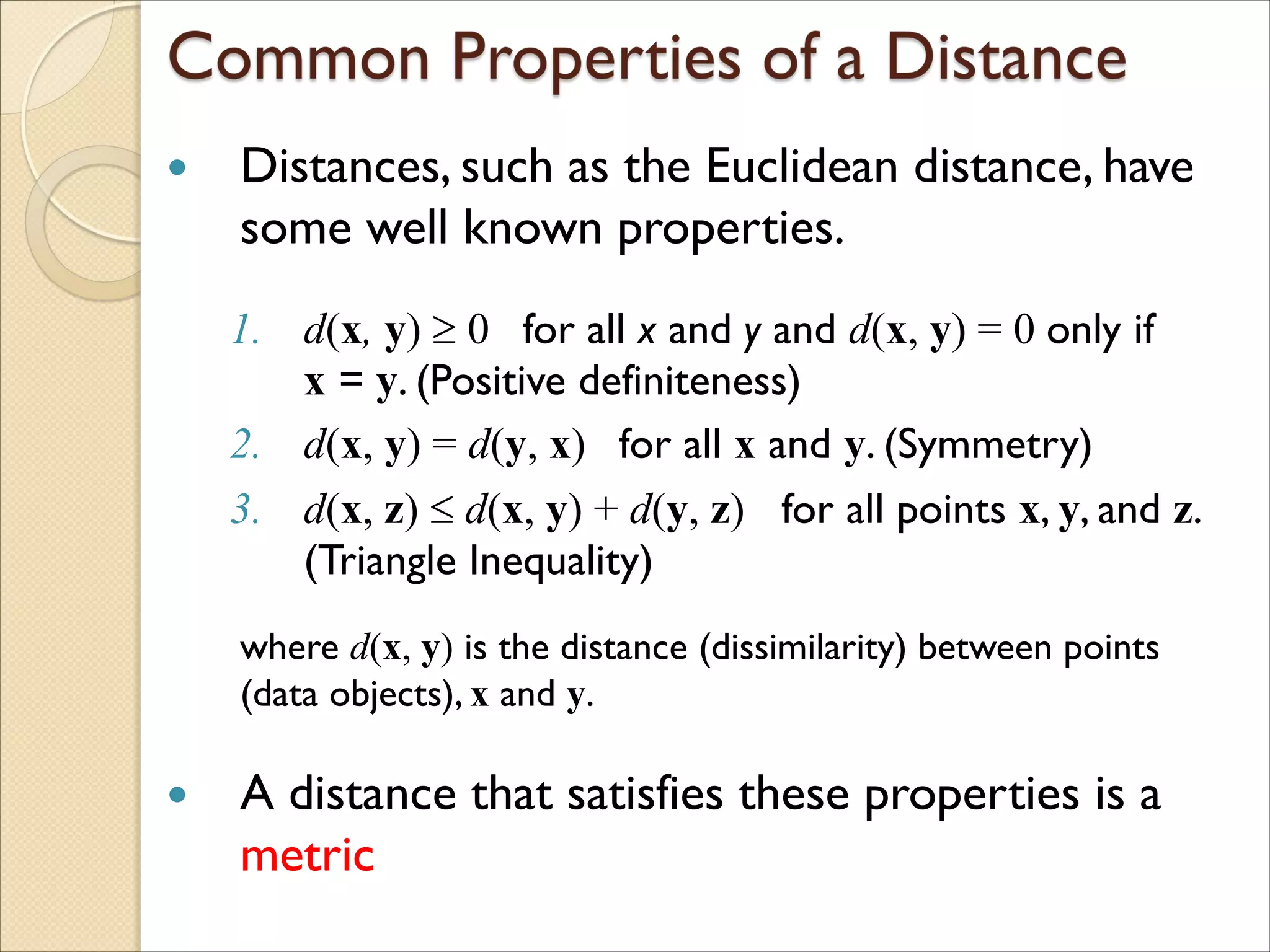
 Distances, such as the Euclidean distance, have
some well known properties.
1. d(x, y)  0 for all x and y and d(x, y) = 0 only if
x = y. (Positive definiteness)
2. d(x, y) = d(y, x) for all x and y. (Symmetry)
3. d(x, z)  d(x, y) + d(y, z) for all points x, y, and z.
(Triangle Inequality)
where d(x, y) is the distance (dissimilarity) between points
(data objects), x and y.
 A distance that satisfies these properties is a
metric

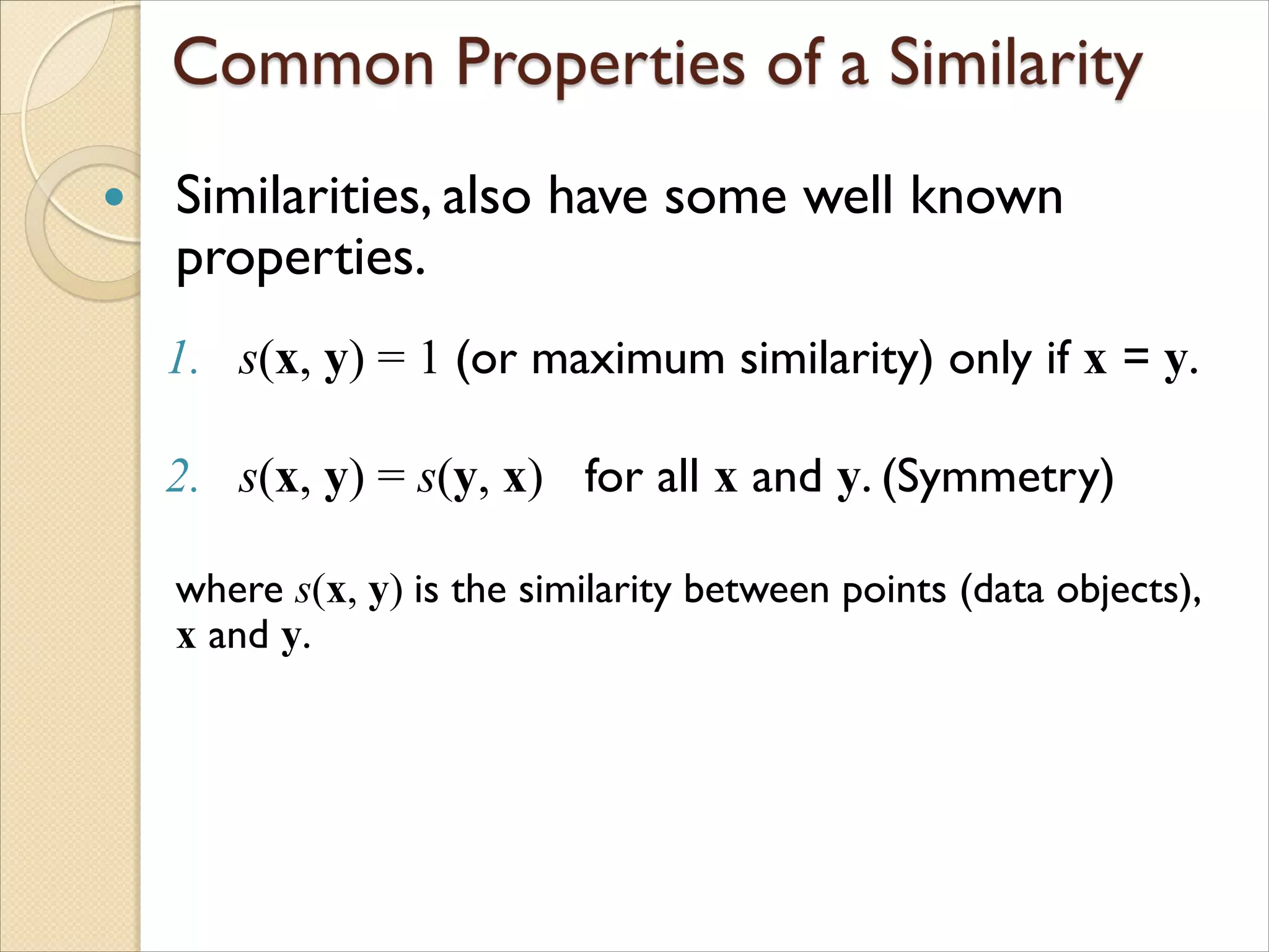
 Similarities, also have some well known
properties.
1. s(x, y) = 1 (or maximum similarity) only if x = y.
2. s(x, y) = s(y, x) for all x and y. (Symmetry)
where s(x, y) is the similarity between points (data objects),
x and y.

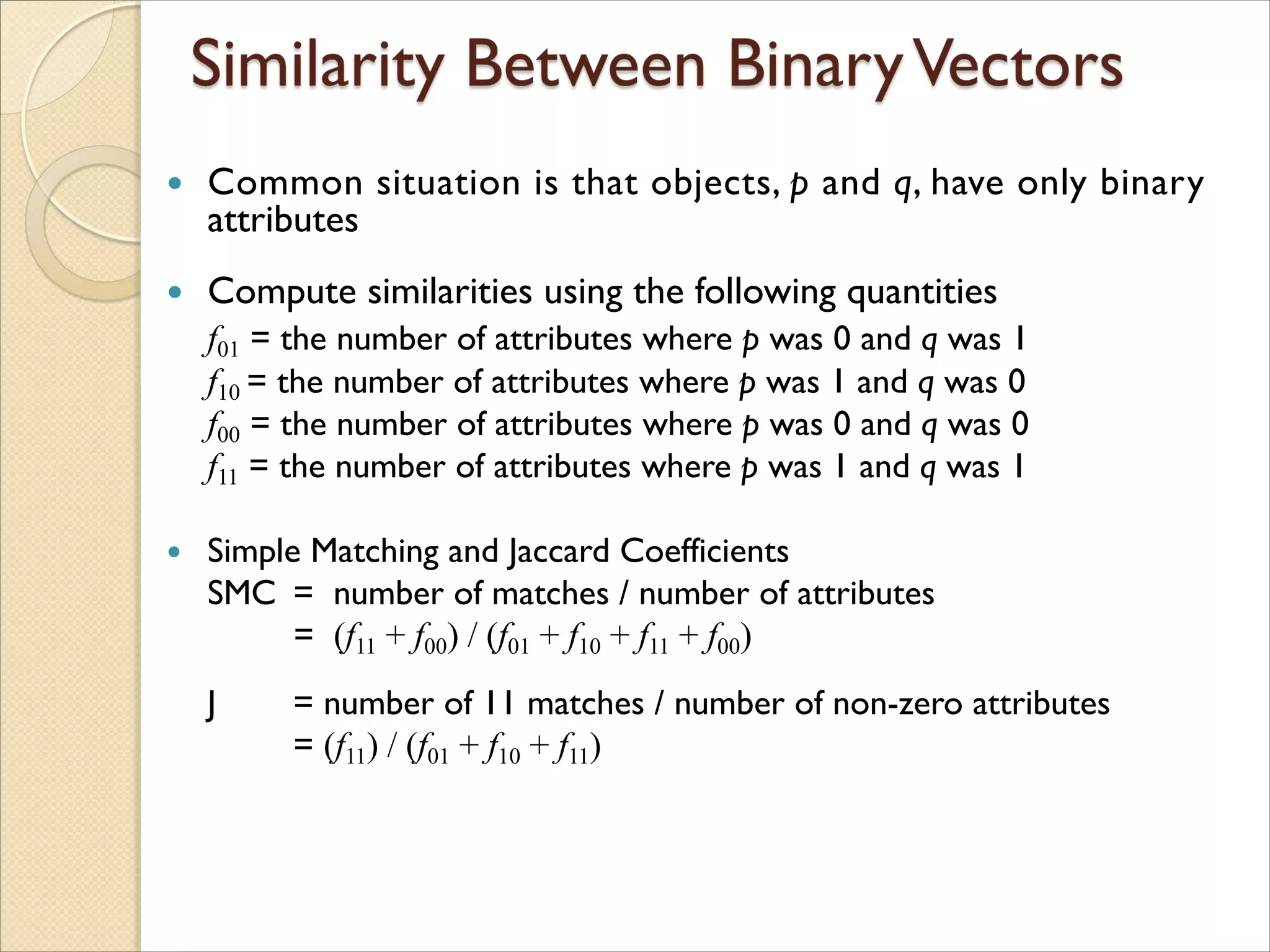
 Common situation is that objects, p and q, have only binary
attributes
 Compute similarities using the following quantities
f01 = the number of attributes where p was 0 and q was 1
 Simple Matching and Jaccard Coefficients
SMC = number of matches / number of attributes
= (f11 + f00) / (f01 + f10 + f11 + f00)
J = number of 11 matches / number of non-zero attributes
= (f11) / (f01 + f10 + f11)

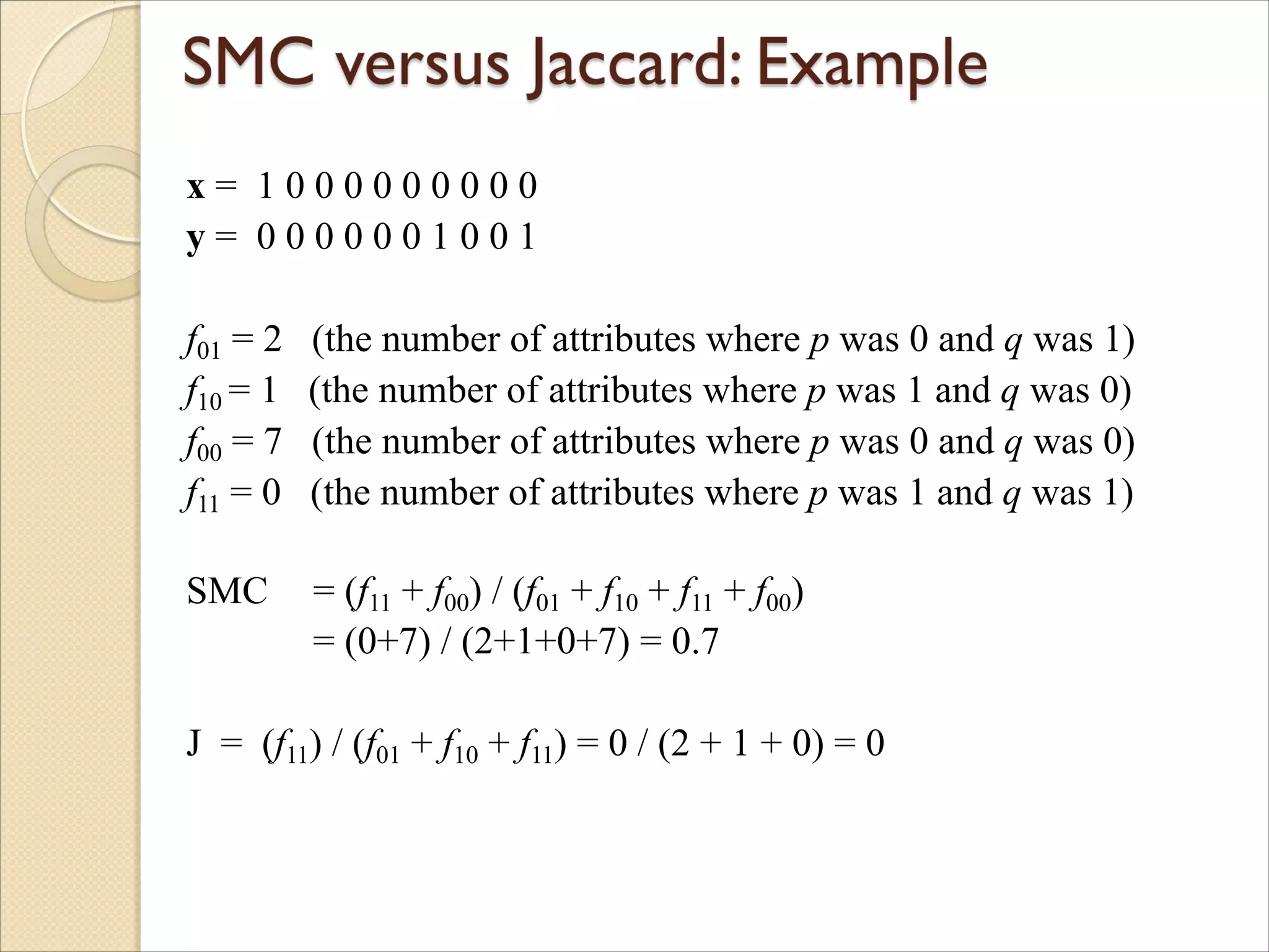
x = 1 0 0 0 0 0 0 0 0 0
y = 0 0 0 0 0 0 1 0 0 1
f01 = 2 (the number of attributes where p was 0 and q was 1)
SMC = (f11 + f00) / (f01 + f10 + f11 + f00)
= (0+7) / (2+1+0+7) = 0.7
J = (f11) / (f01 + f10 + f11) = 0 / (2 + 1 + 0) = 0

 Domain of application
◦ Similarity measures tend to be specific to the type of
attribute and data
◦ Record data, images, graphs, sequences, 3D-protein structure,
etc. tend to have different measures
 However, one can talk about various properties that
you would like a proximity measure to have
◦ Symmetry is a common one
◦ Tolerance to noise and outliers is another
◦ Ability to find more types of patterns?
◦ Many others possible
 The measure must be applicable to the data and
produce results that agree with domain knowledge

 Information theory is a well-developed and
fundamental disciple with broad applications
 Some similarity measures are based on
information theory
◦ Mutual information in various versions
◦ Maximal Information Coefficient (MIC) and
related measures
◦ General and can handle non-linear relationships
◦ Can be complicated and time intensive to
compute

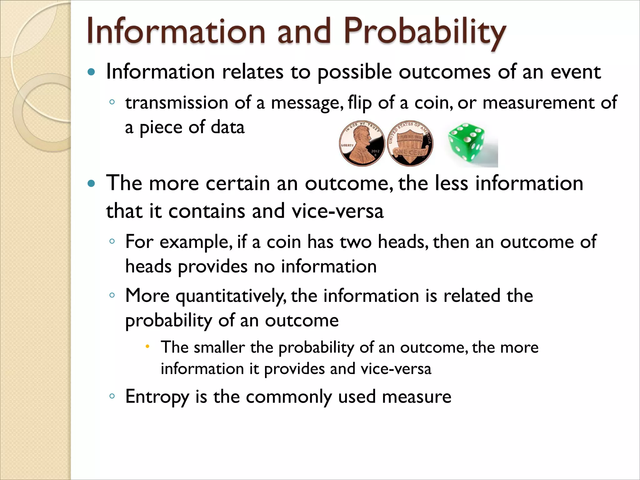
 Information relates to possible outcomes of an event
◦ transmission of a message, flip of a coin, or measurement of
a piece of data
 The more certain an outcome, the less information
that it contains and vice-versa
◦ For example, if a coin has two heads, then an outcome of
heads provides no information
◦ More quantitatively, the information is related the
probability of an outcome
 The smaller the probability of an outcome, the more
information it provides and vice-versa
◦ Entropy is the commonly used measure

 Measures the degree to which data objects are close to
each other in a specified area
 The notion of density is closely related to that of
proximity
 Concept of density is typically used for clustering and
anomaly detection
 Examples:
◦ Euclidean density
 Euclidean density = number of points per unit volume
◦ Probability density
 Estimate what the distribution of the data looks like
◦ Graph-based density
 Connectivity

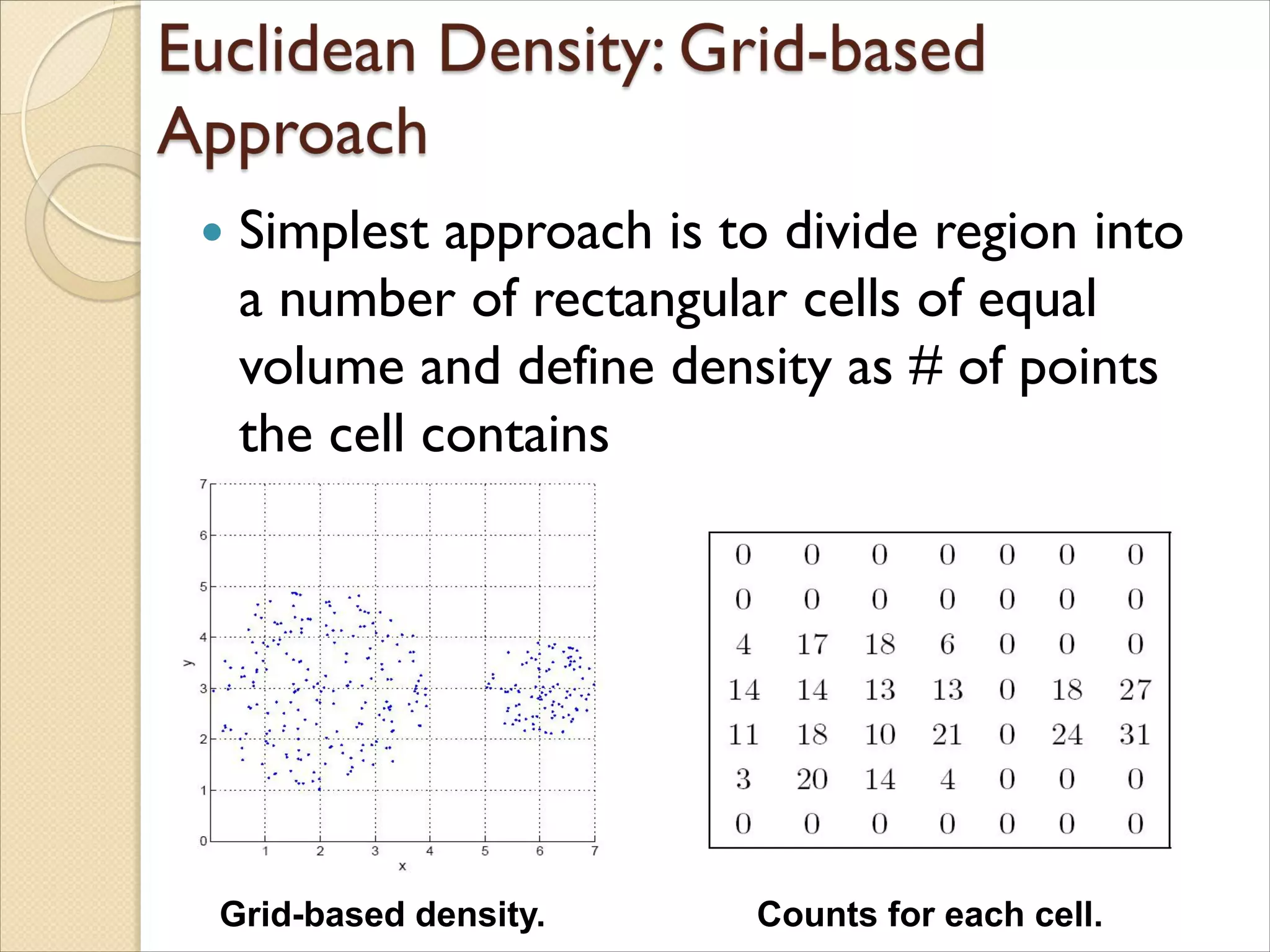
 Simplest approach is to divide region into
a number of rectangular cells of equal
volume and define density as # of points
the cell contains
Grid-based density. Counts for each cell.

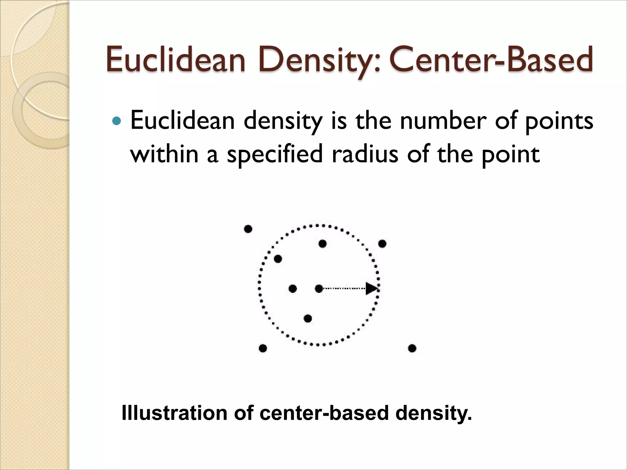
 Euclidean density is the number of points
within a specified radius of the point
Illustration of center-based density.

 Aggregation
 Sampling
 Dimensionality Reduction
 Feature subset selection
 Feature creation
 Discretization and Binarization
 Attribute Transformation

 Combining two or more attributes (or
objects) into a single attribute (or object)
 Purpose
◦ Data reduction
 Reduce the number of attributes or objects
◦ Change of scale
 Cities aggregated into regions, states, countries, etc.
 Days aggregated into weeks, months, or years
◦ More “stable” data
 Aggregated data tends to have less variability

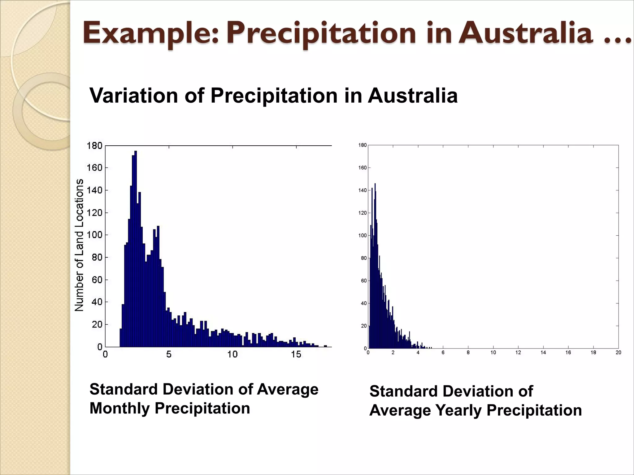
 This example is based on precipitation in Australia
from the period 1982 to 1993.
The next slide shows
◦ A histogram for the standard deviation of average monthly
precipitation for 3,030 0.5◦ by 0.5◦ grid cells in Australia,
and
◦ A histogram for the standard deviation of the average yearly
precipitation for the same locations.
 The average yearly precipitation has less variability
than the average monthly precipitation.
 All precipitation measurements (and their standard
deviations) are in centimeters.

Standard Deviation of Average
Monthly Precipitation
Standard Deviation of
Average Yearly Precipitation
Variation of Precipitation in Australia

 Sampling is the main technique employed for data
reduction.
◦ It is often used for both the preliminary investigation
of the data and the final data analysis.
 Statisticians often sample because obtaining the
entire set of data of interest is too expensive or
time consuming.
 Sampling is typically used in data mining because
processing the entire set of data of interest is too
expensive or time consuming.

 The key principle for effective sampling is
the following:
◦ Using a sample will work almost as well as using
the entire data set, if the sample is
representative
◦ A sample is representative if it has
approximately the same properties (of interest)
as the original set of data

8000 points 2000 Points 500 Points

 Simple Random Sampling
◦ There is an equal probability of selecting any particular
item
◦ Sampling without replacement
 As each item is selected, it is removed from the population
◦ Sampling with replacement
 Objects are not removed from the population as they are
selected for the sample.
 In sampling with replacement, the same object can be
picked up more than once
 Stratified sampling
◦ Split the data into several partitions; then draw random
samples from each partition

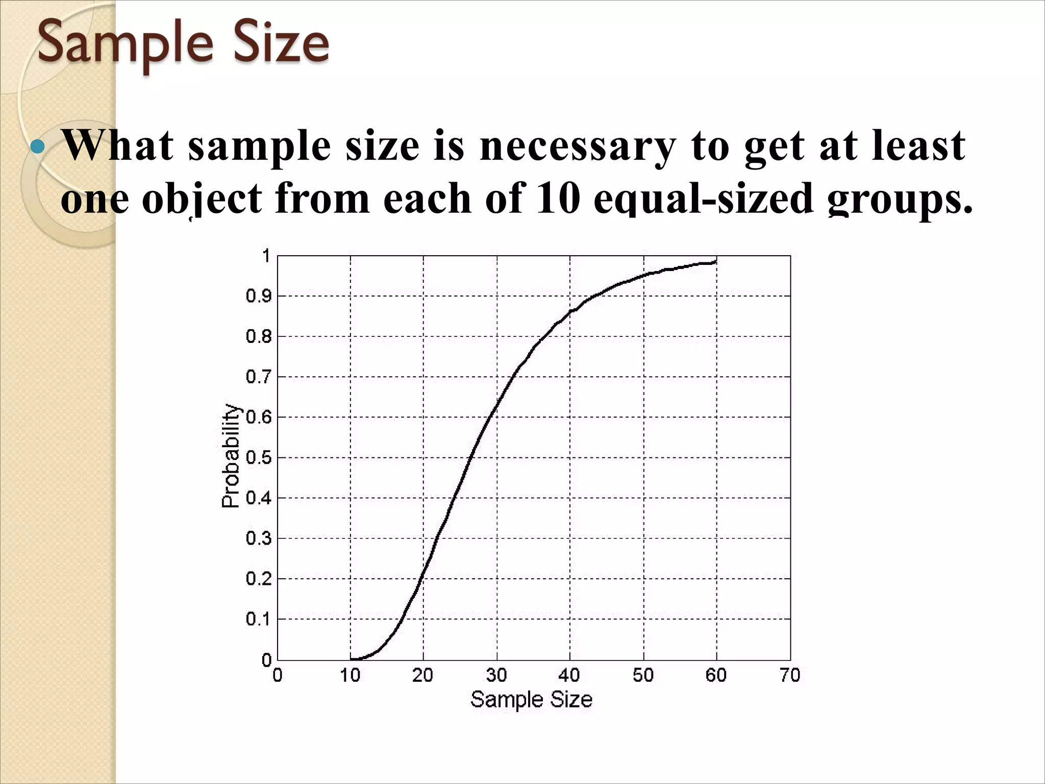
 What sample size is necessary to get at least
one object from each of 10 equal-sized groups.

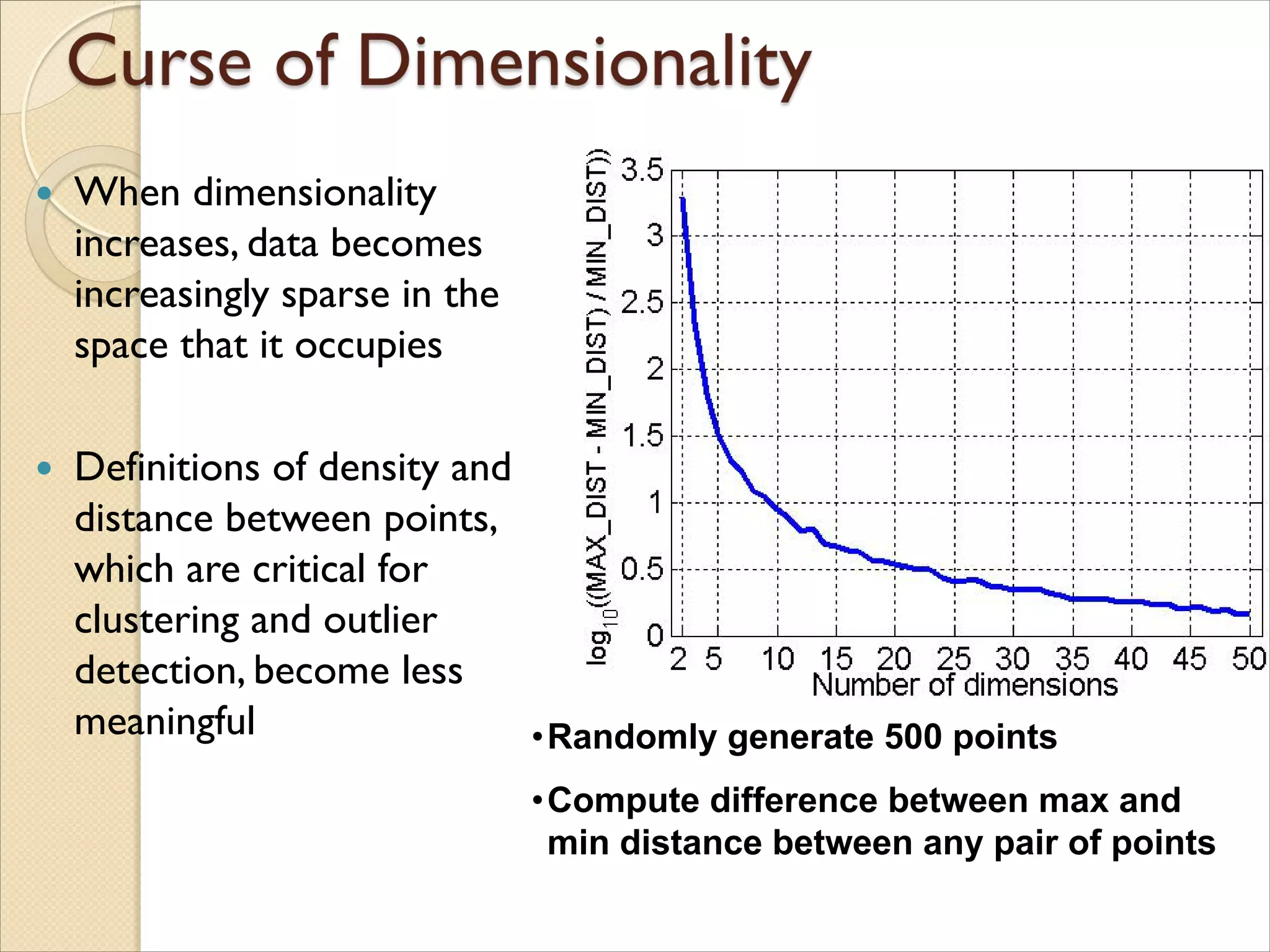
 When dimensionality
increases, data becomes
increasingly sparse in the
space that it occupies
 Definitions of density and
distance between points,
which are critical for
clustering and outlier
detection, become less
meaningful •Randomly generate 500 points
•Compute difference between max and
min distance between any pair of points

 Purpose:
◦ Avoid curse of dimensionality
◦ Reduce amount of time and memory required
by data mining algorithms
◦ Allow data to be more easily visualized
◦ May help to eliminate irrelevant features or
reduce noise
 Techniques
◦ Principal Components Analysis (PCA)
◦ SingularValue Decomposition
◦ Others: supervised and non-linear techniques

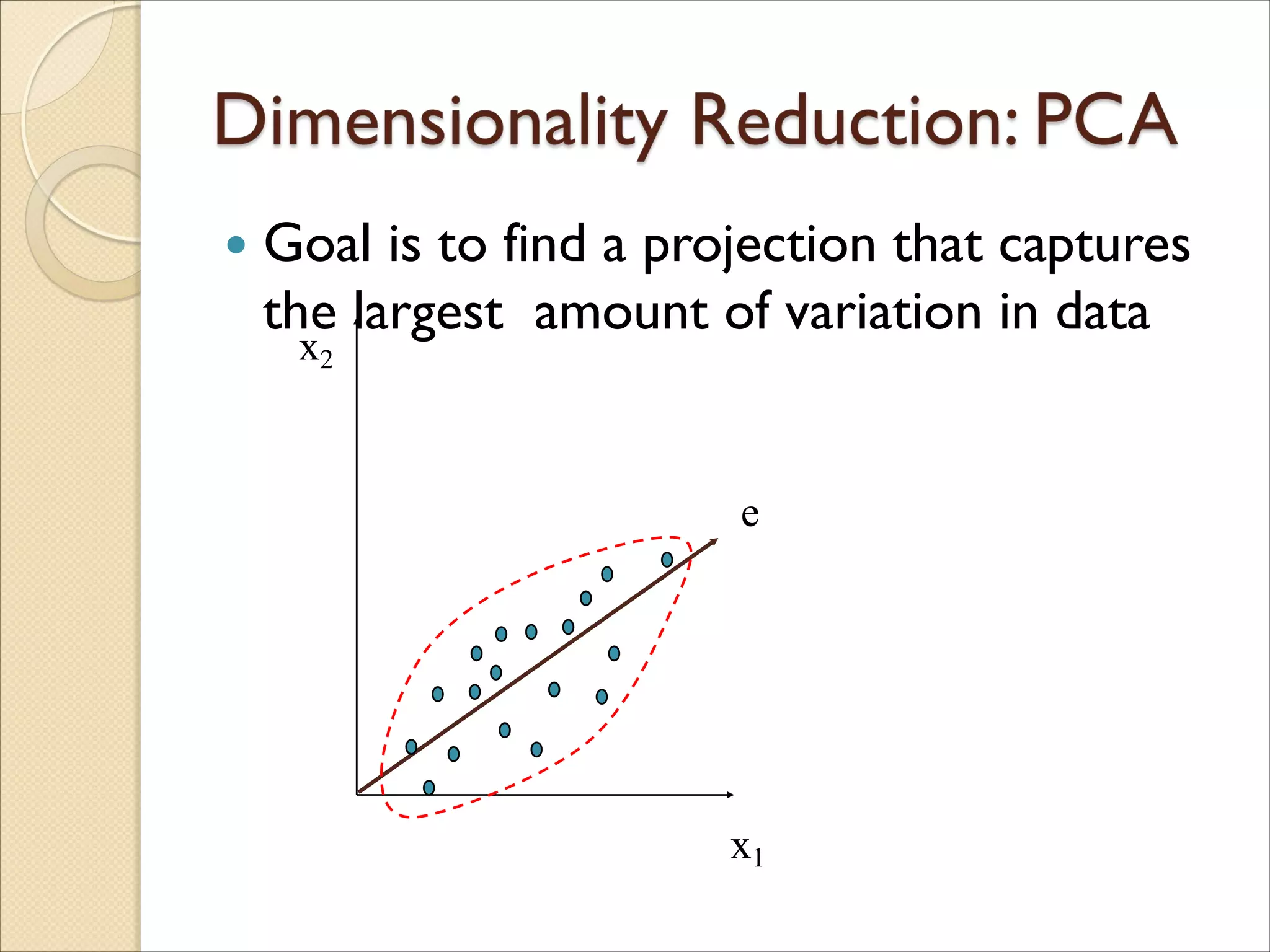
 Goal is to find a projection that captures
the largest amount of variation in data
x2
x1
e

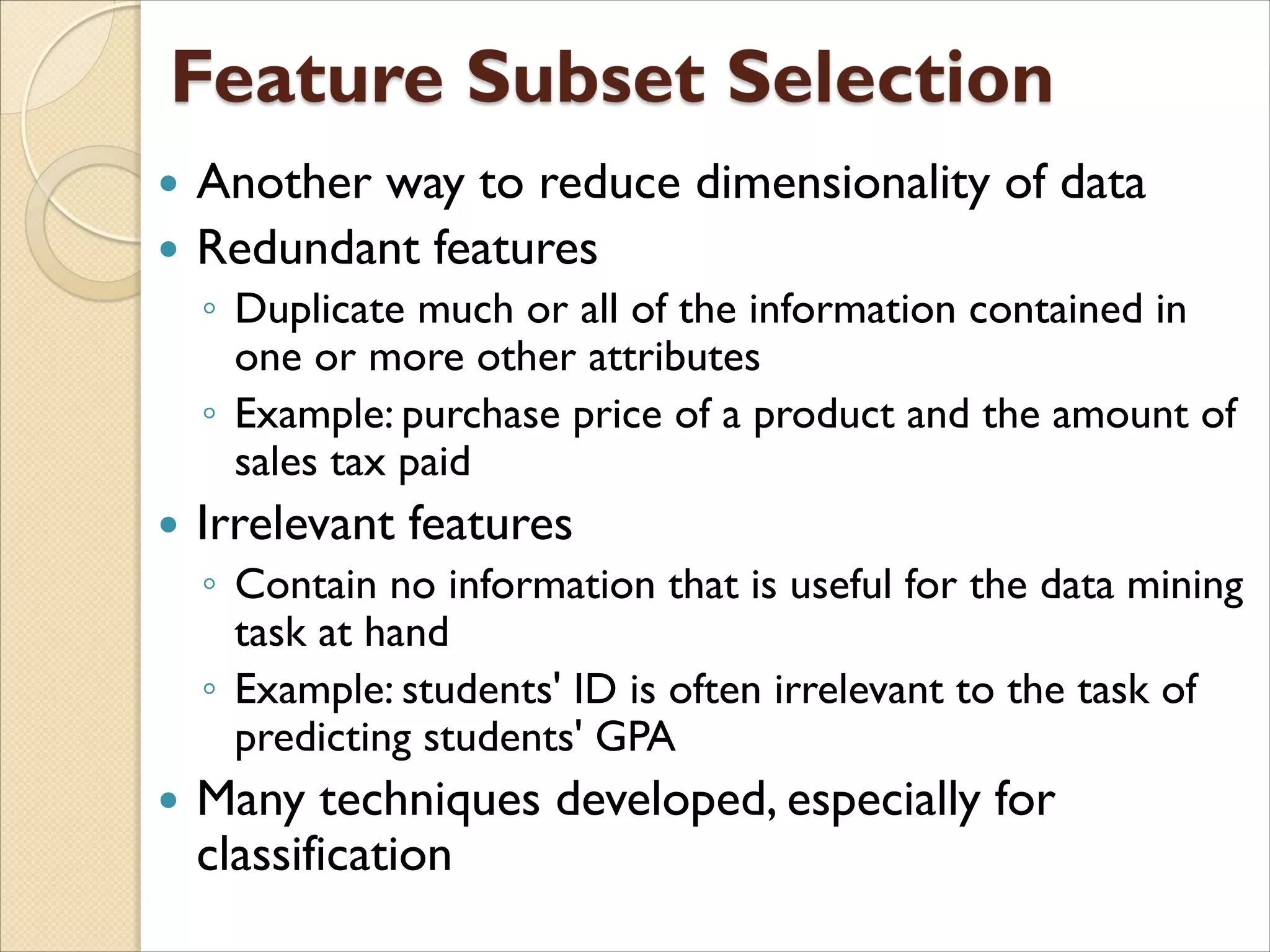
 Another way to reduce dimensionality of data
 Redundant features
◦ Duplicate much or all of the information contained in
one or more other attributes
◦ Example: purchase price of a product and the amount of
sales tax paid
 Irrelevant features
◦ Contain no information that is useful for the data mining
task at hand
◦ Example: students' ID is often irrelevant to the task of
predicting students' GPA
 Many techniques developed, especially for
classification

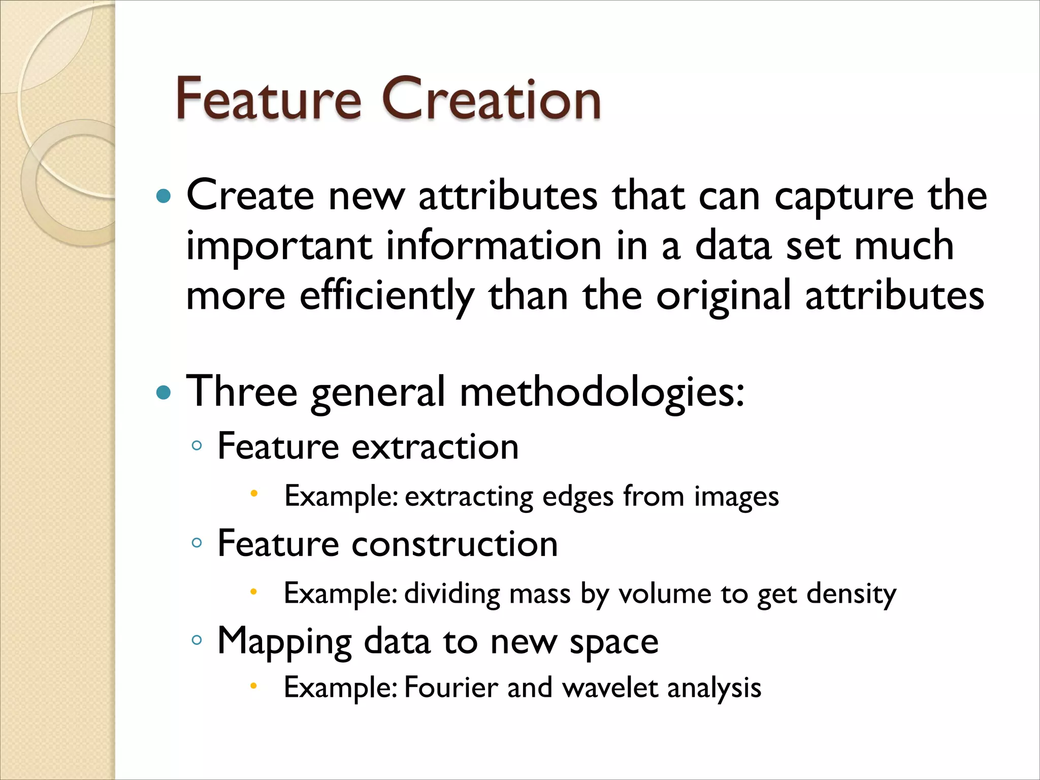
 Create new attributes that can capture the
important information in a data set much
more efficiently than the original attributes
 Three general methodologies:
◦ Feature extraction
 Example: extracting edges from images
◦ Feature construction
 Example: dividing mass by volume to get density
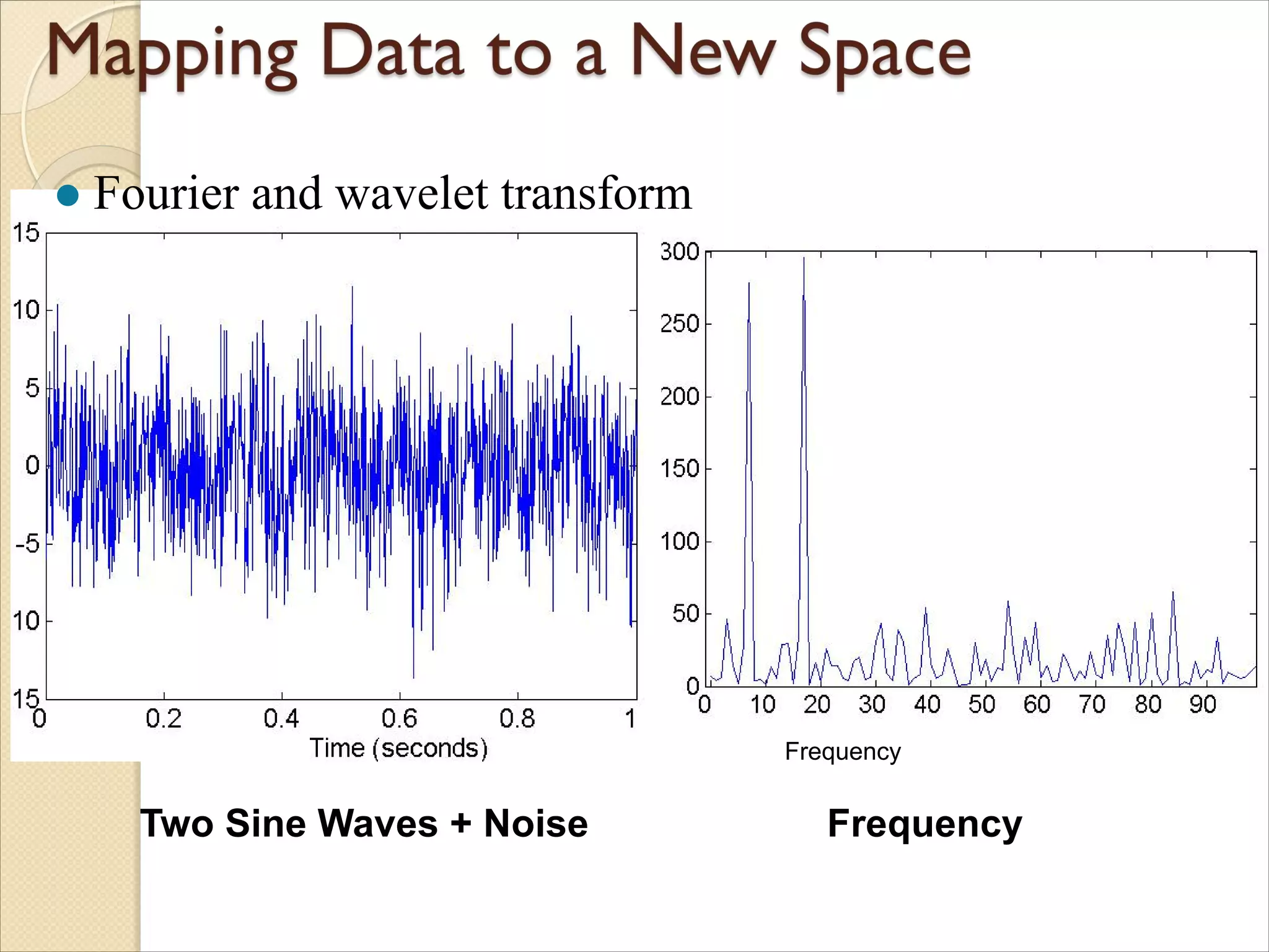
◦ Mapping data to new space
 Example: Fourier and wavelet analysis

Two Sine Waves + Noise Frequency
l Fourier and wavelet transform
Frequency

 Discretization is the process of converting a
continuous attribute into an ordinal
attribute
◦ A potentially infinite number of values are
mapped into a small number of categories
◦ Discretization is commonly used in classification
◦ Many classification algorithms work best if both the
independent and dependent variables have only a
few values
◦ We give an illustration of the usefulness of
discretization using the Iris data set

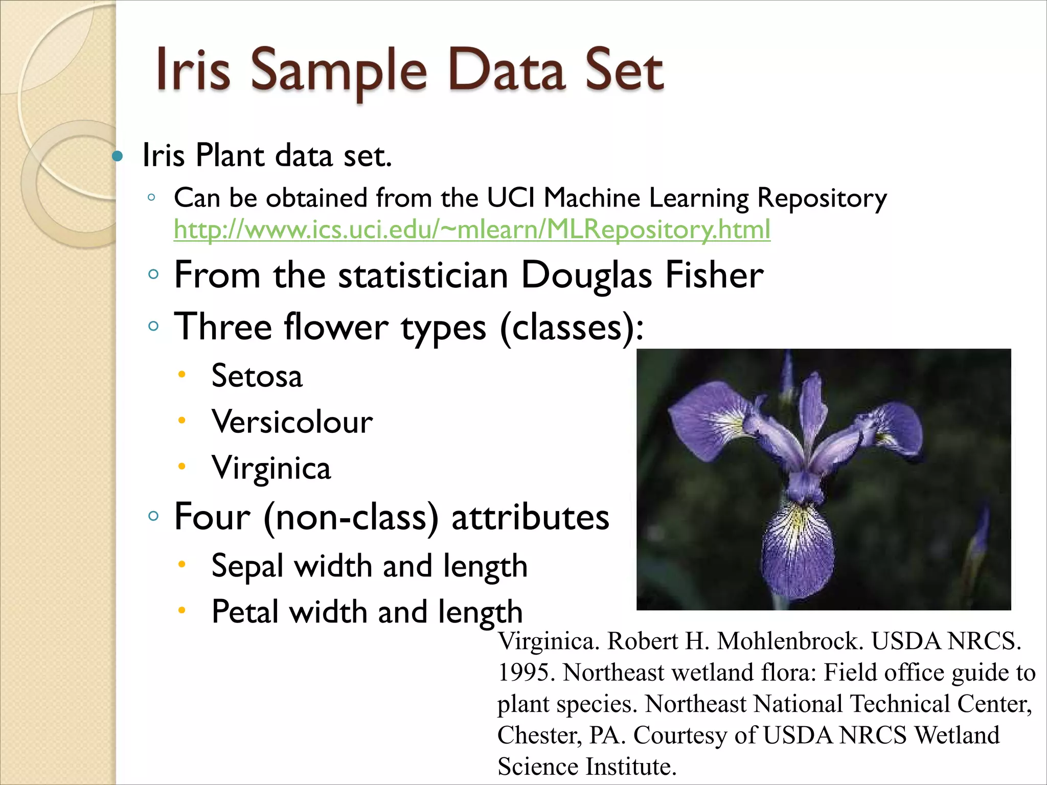
 Iris Plant data set.
◦ Can be obtained from the UCI Machine Learning Repository
http://www.ics.uci.edu/~mlearn/MLRepository.html
◦ From the statistician Douglas Fisher
◦ Three flower types (classes):
 Setosa
 Versicolour
 Virginica
◦ Four (non-class) attributes
 Sepal width and length
 Petal width and length
Virginica. Robert H. Mohlenbrock. USDA NRCS.
1995. Northeast wetland flora: Field office guide to
plant species. Northeast National Technical Center,
Chester, PA. Courtesy of USDA NRCS Wetland
Science Institute.

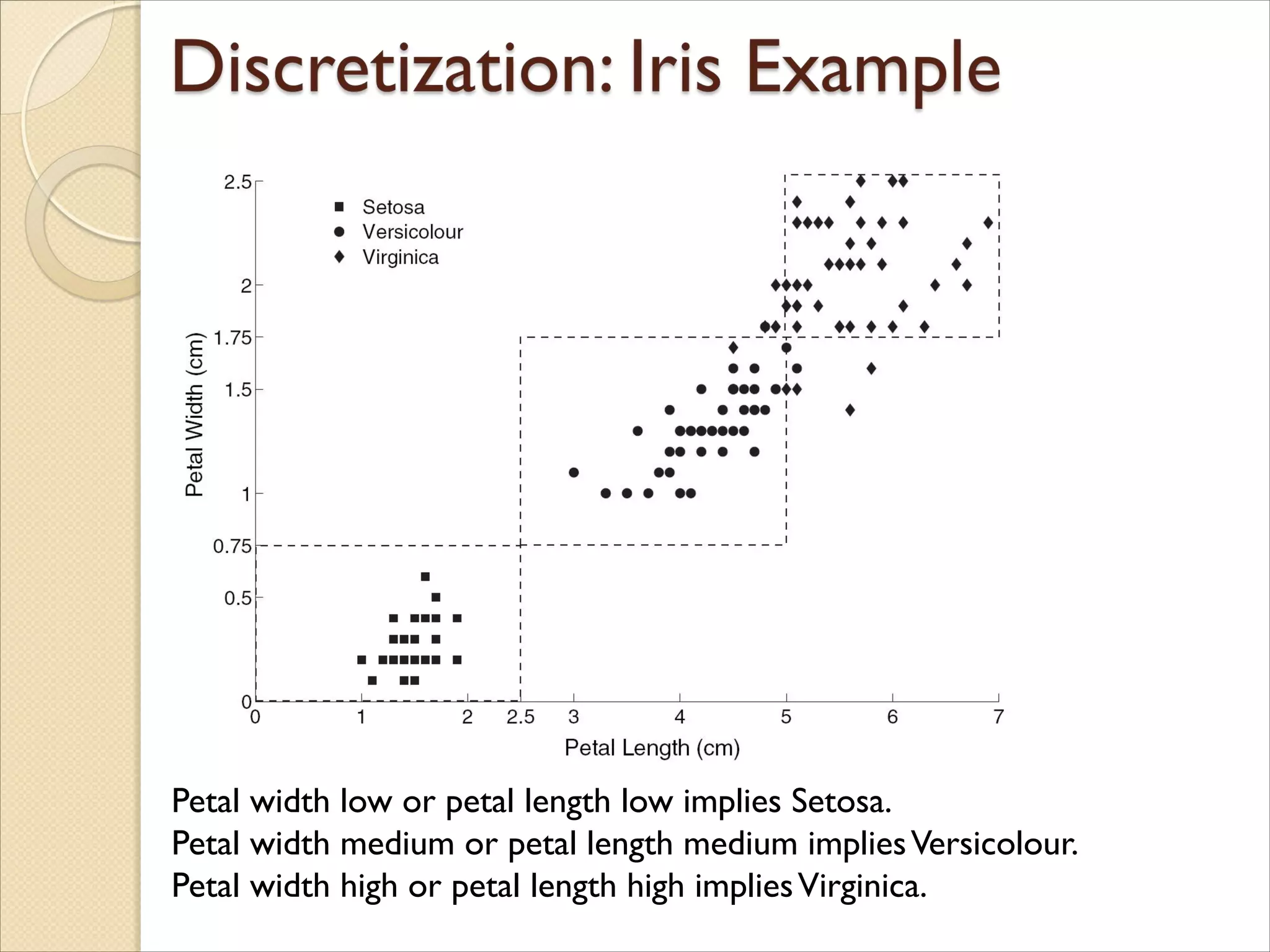
Petal width low or petal length low implies Setosa.
Petal width medium or petal length medium impliesVersicolour.
Petal width high or petal length high impliesVirginica.

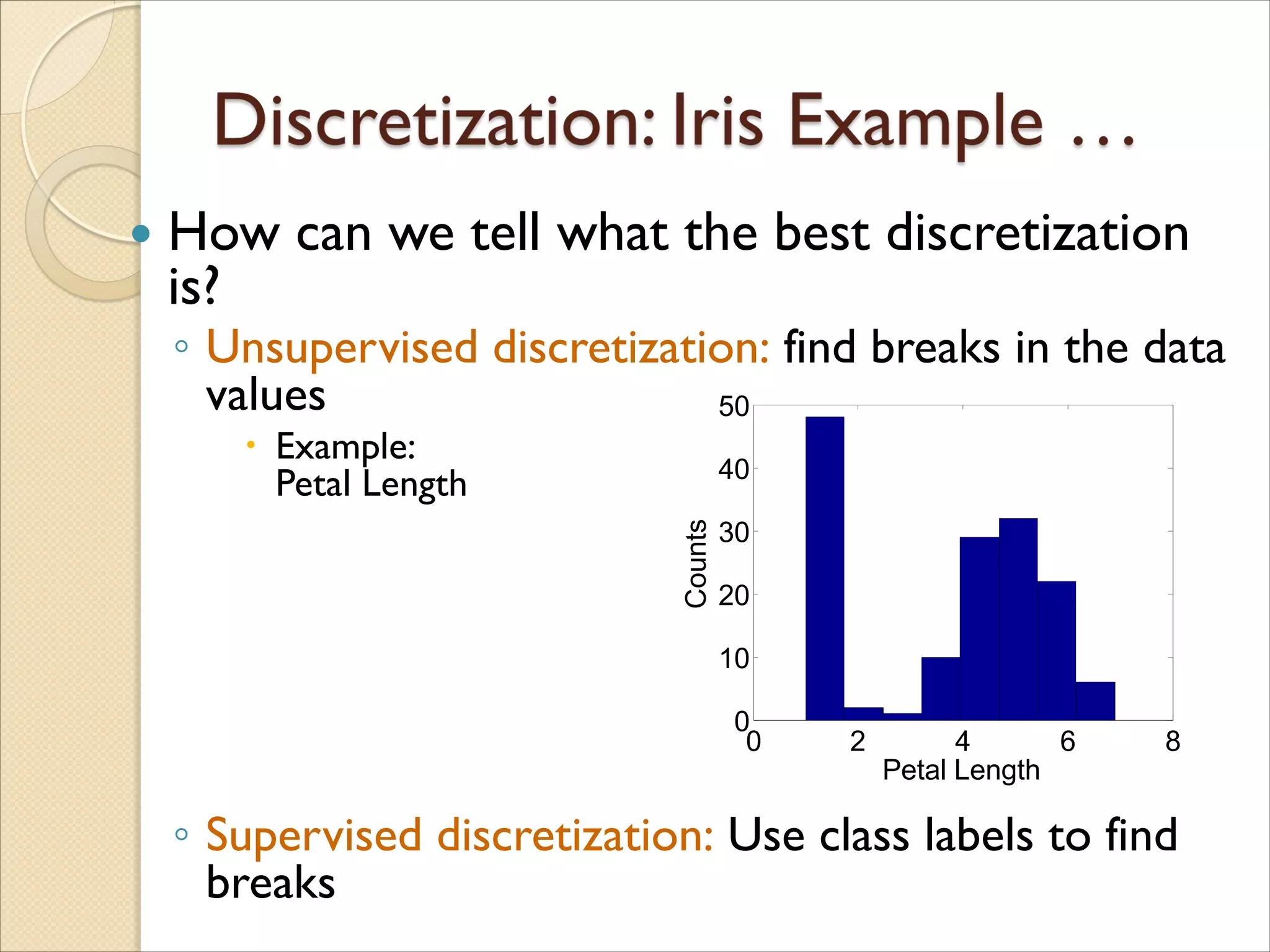
 How can we tell what the best discretization
is?
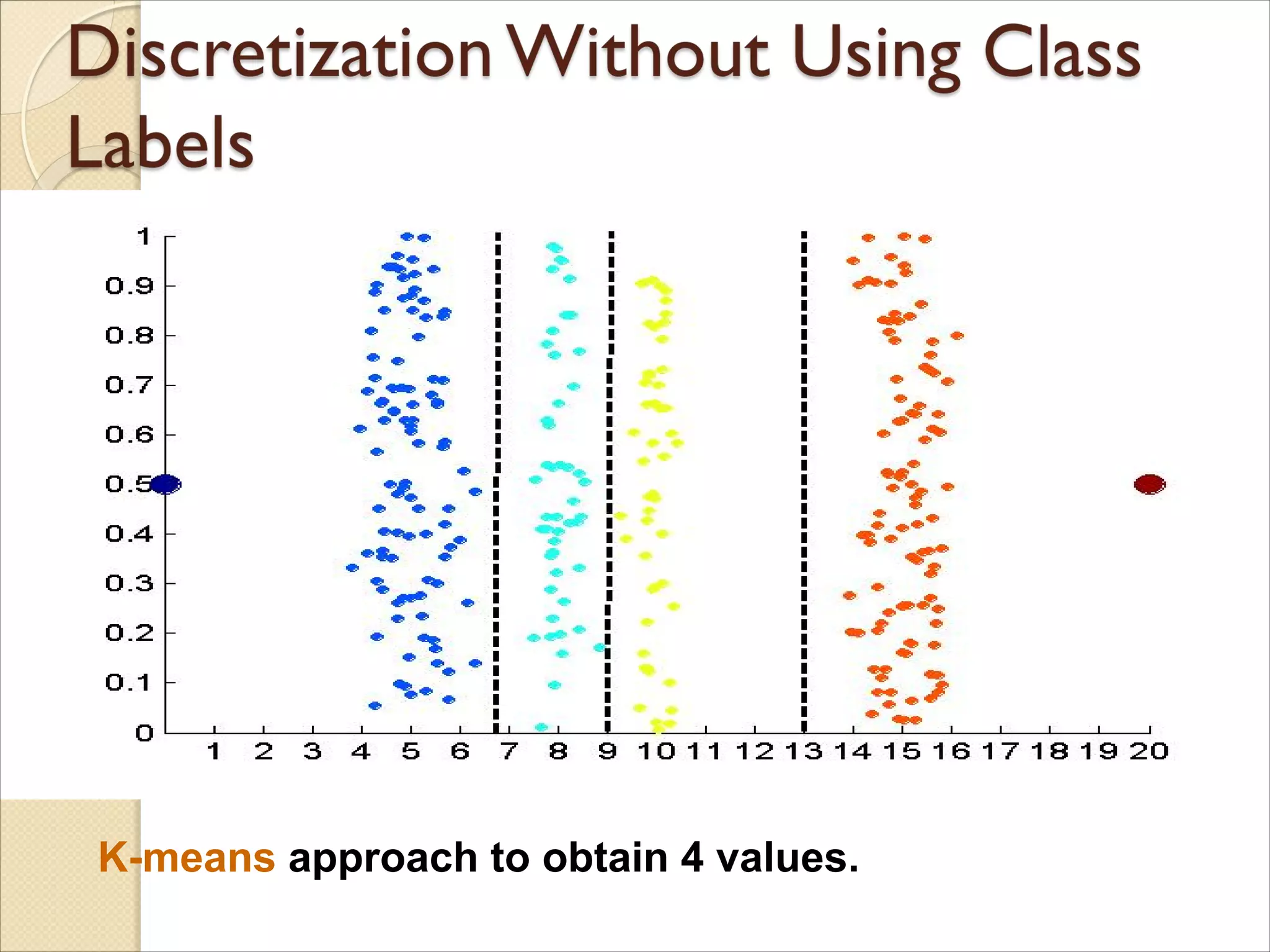
◦ Unsupervised discretization: find breaks in the data
values
 Example:
Petal Length
◦ Supervised discretization: Use class labels to find
breaks
0 2 4 6 8
0
10
20
30
40
50
Petal Length
Counts

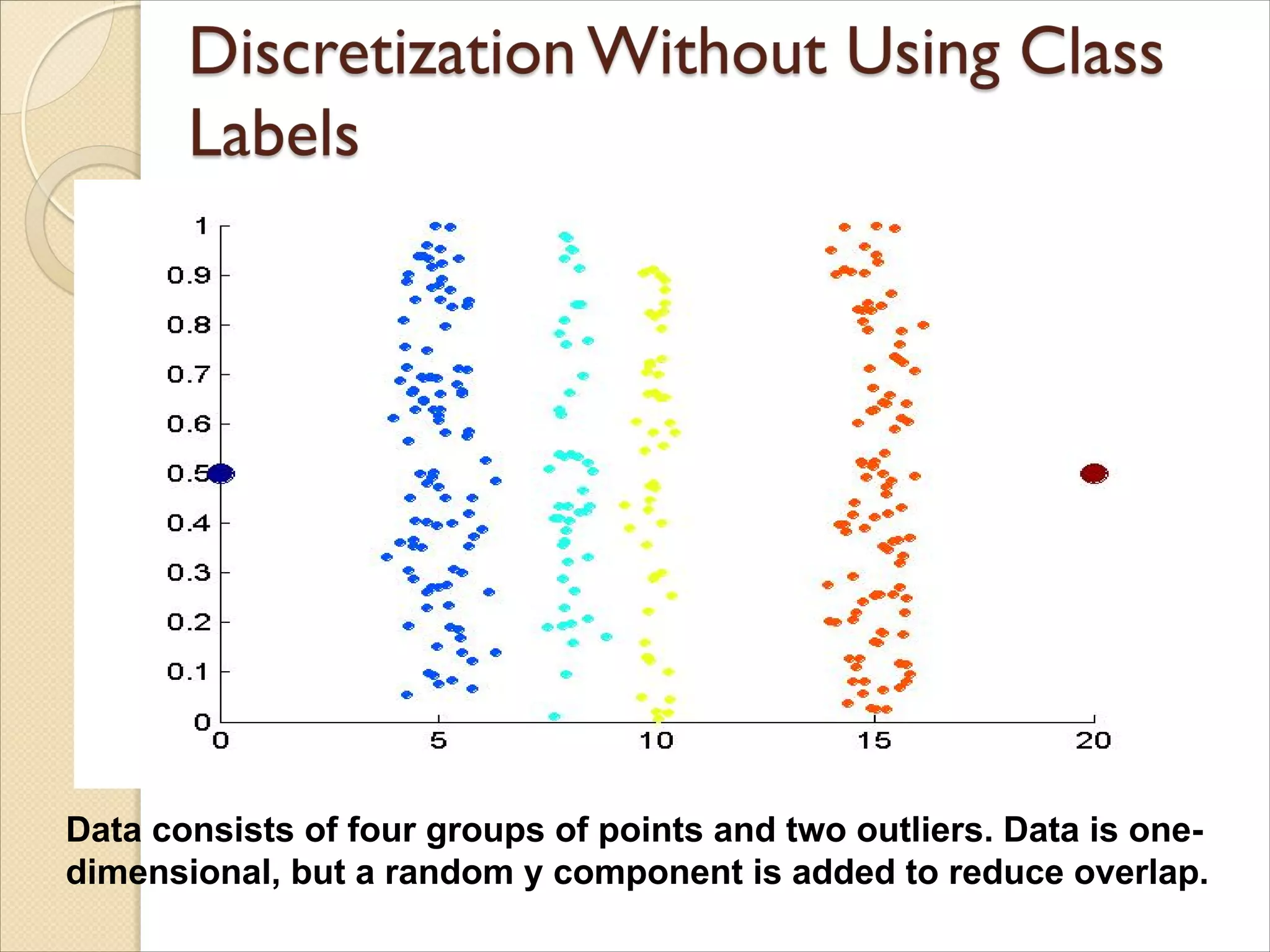
Data consists of four groups of points and two outliers. Data is one-
dimensional, but a random y component is added to reduce overlap.

Equal interval width approach used to obtain 4 values.

Equal frequency approach used to obtain 4 values.

K-means approach to obtain 4 values.

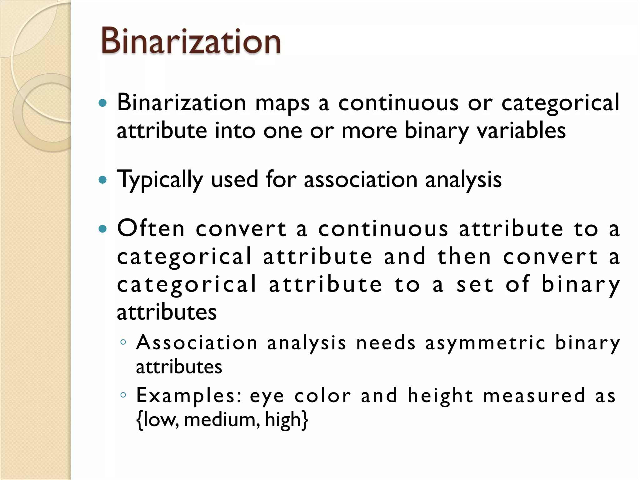
 Binarization maps a continuous or categorical
attribute into one or more binary variables
 Typically used for association analysis
 Often convert a continuous attribute to a
categorical attribute and then convert a
categorical attribute to a set of binary
attributes
◦ Association analysis needs asymmetric binary
attributes
◦ Examples: eye color and height measured as
{low, medium, high}

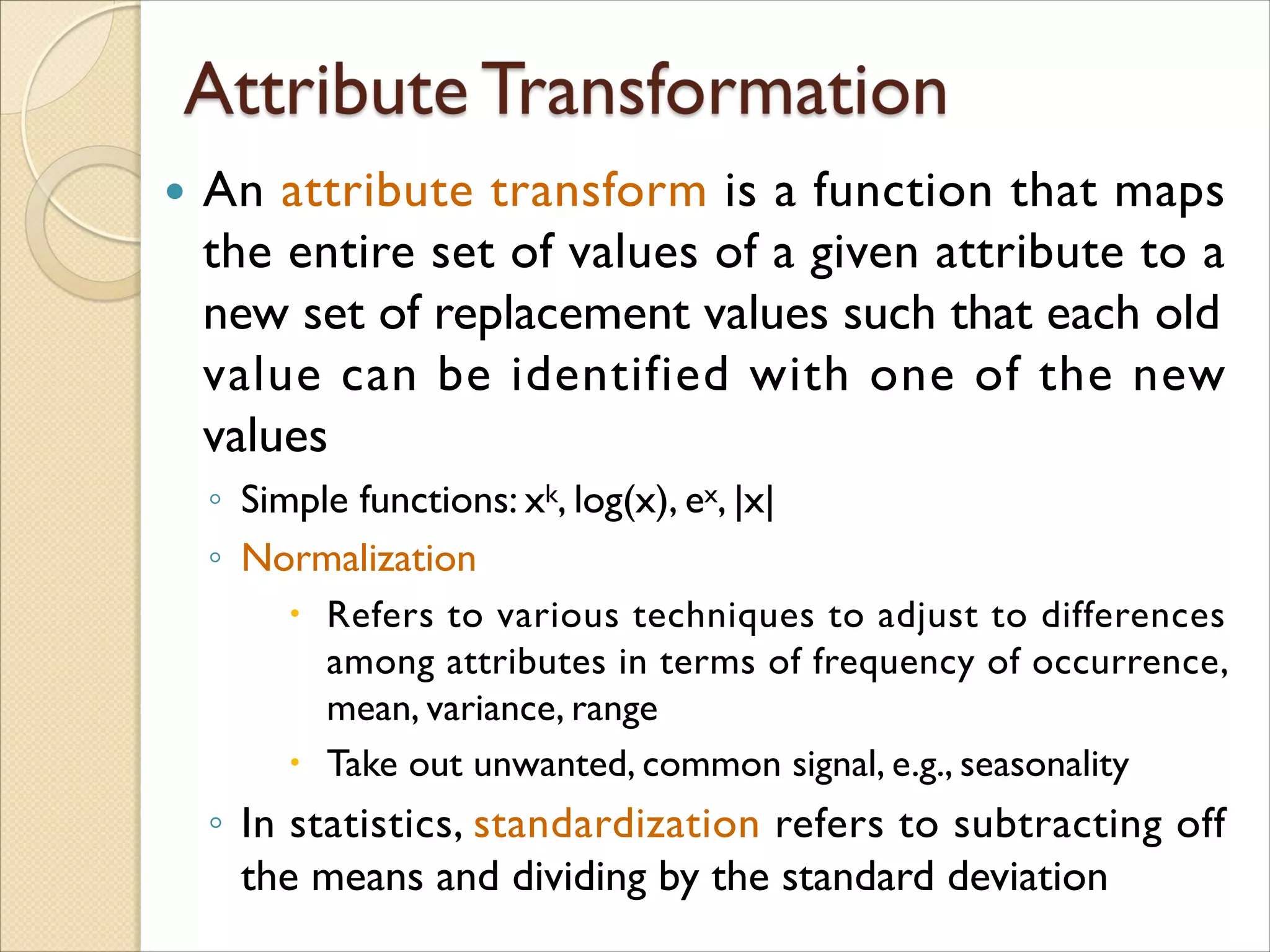
 An attribute transform is a function that maps
the entire set of values of a given attribute to a
new set of replacement values such that each old
value can be identified with one of the new
values
◦ Simple functions: xk, log(x), ex, |x|
◦ Normalization
 Refers to various techniques to adjust to differences
among attributes in terms of frequency of occurrence,
mean, variance, range
 Take out unwanted, common signal, e.g., seasonality
◦ In statistics, standardization refers to subtracting off
the means and dividing by the standard deviation

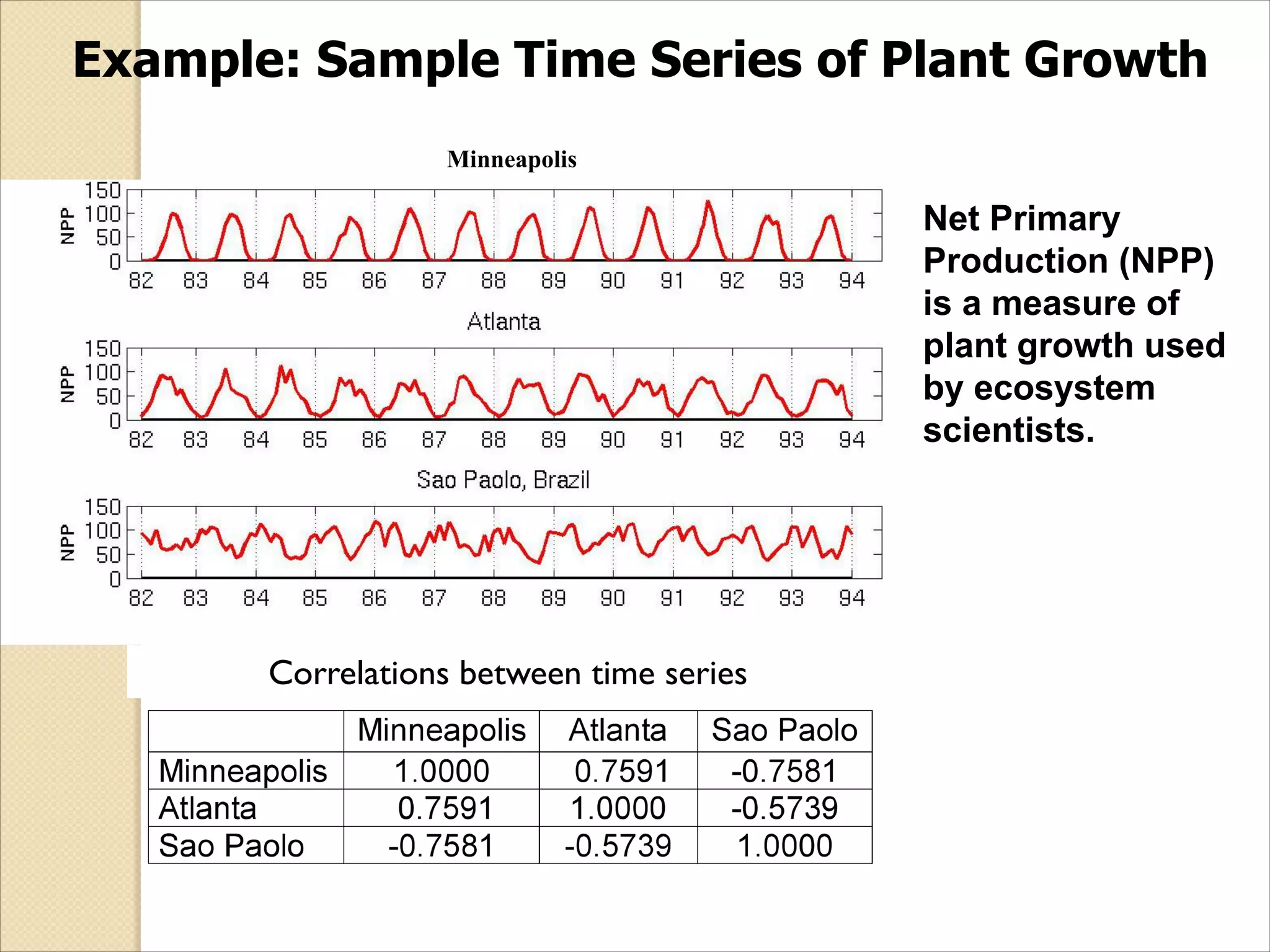
Example: Sample Time Series of Plant Growth
Correlations between time series
Minneapolis
Correlations between time series
Net Primary
Production (NPP)
is a measure of
plant growth used
by ecosystem
scientists.

Lect 2 getting to know your data

Recommended

Recommended

More Related Content

What's hot

What's hot (20)

Similar to Lect 2 getting to know your data

Similar to Lect 2 getting to know your data (20)

More from hktripathy

More from hktripathy (17)

Recently uploaded

Recently uploaded (20)

Lect 2 getting to know your data