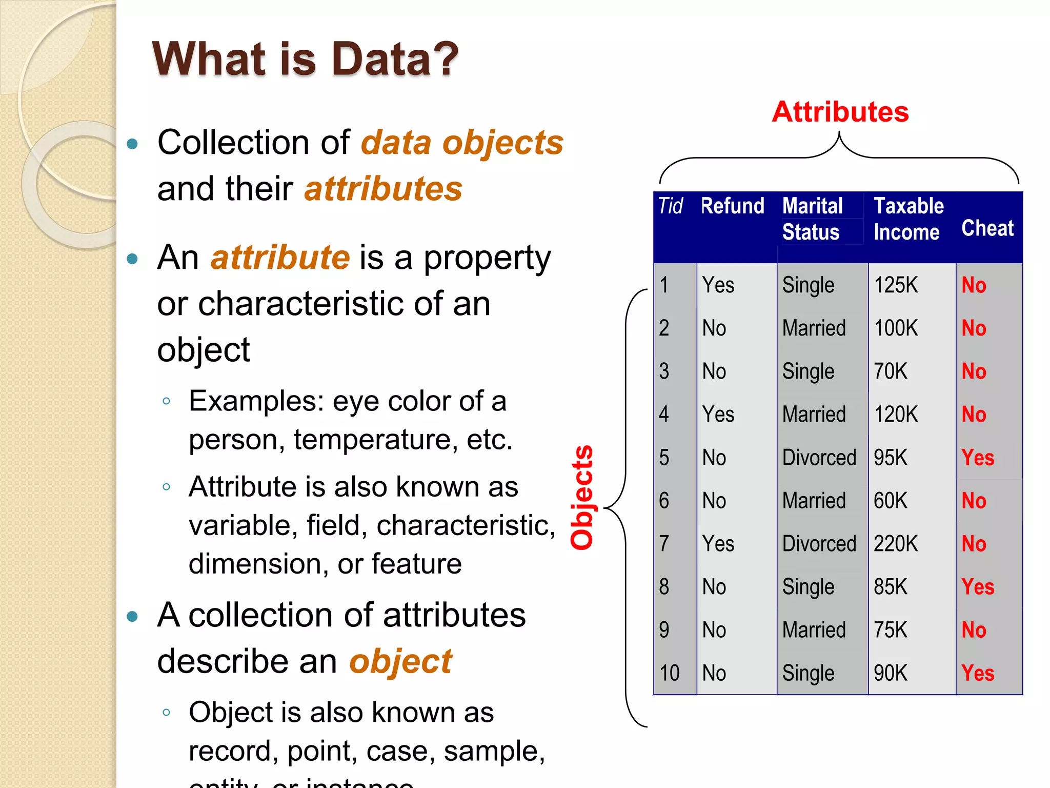
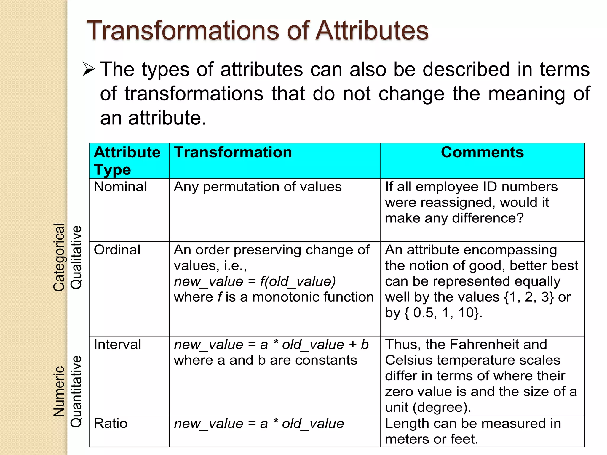
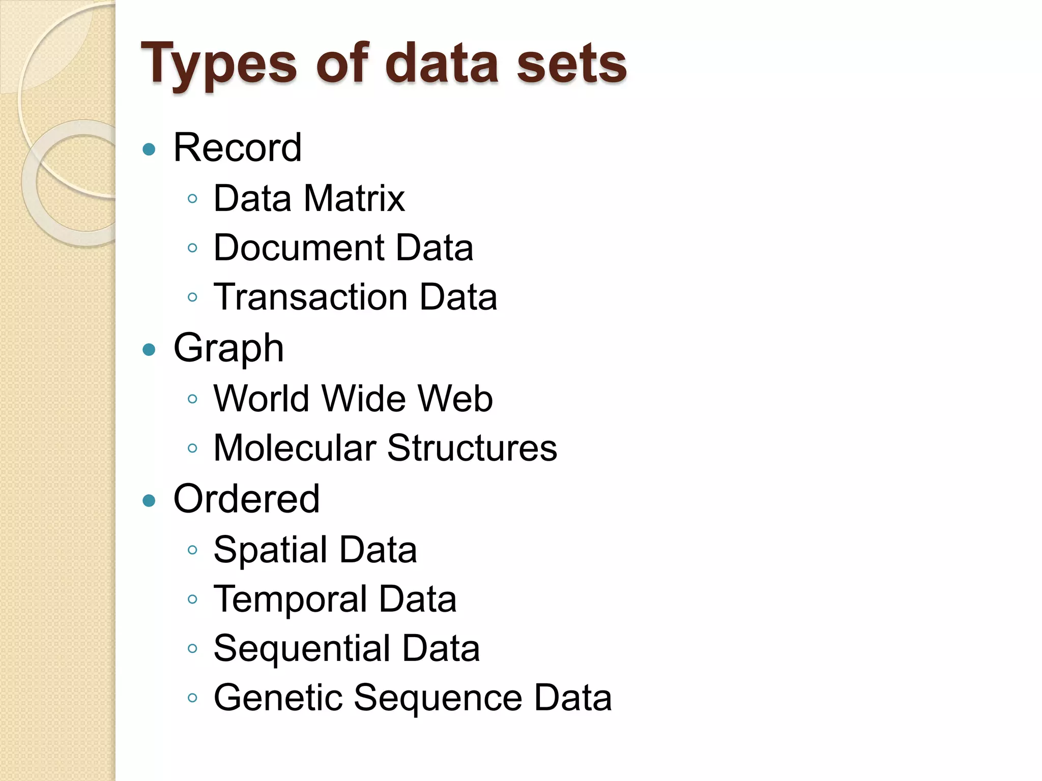
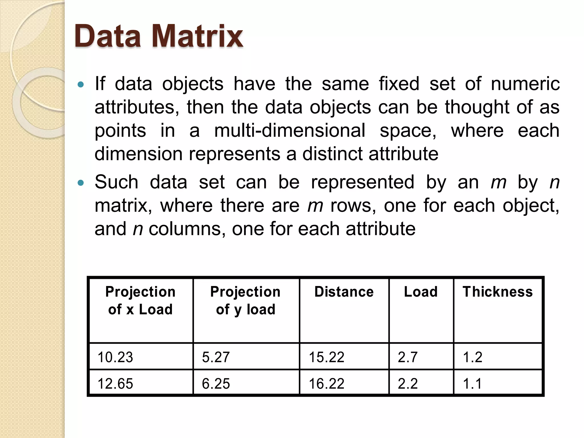
This document provides an overview of getting to know data through data mining and data warehousing. It defines key concepts like data objects, attributes, attribute types, data sets, and data quality issues. Data objects are described by a set of attributes, which can be qualitative like nominal or ordinal, or quantitative like interval or ratio scaled. Different types of data sets are discussed including data matrices, documents, transactions, graphs, and ordered data. Common data quality problems addressed are noise, outliers, missing values, and duplicate data. Methods for measuring similarity and dissimilarity between data objects are also introduced.

1. Getting to Know Your Data
DATA MINING AND
DATA WAREHOUSING
CS- 6301 (Cr-4)
Dr. Hrudaya Kumar Tripathy

2. Outline
 Data Objects and Attribute Types
 Basic Statistical Descriptions of Data
 Data Visualization
 Measuring Data Similarity and Dissimilarity
 Summary

3. What is Data?
 Collection of data objects
and their attributes
 An attribute is a property
or characteristic of an
object
◦ Examples: eye color of a
person, temperature, etc.
◦ Attribute is also known as
variable, field, characteristic,
dimension, or feature
 A collection of attributes
describe an object
◦ Object is also known as
record, point, case, sample,
Tid Refund Marital
Status
Taxable
Income Cheat
1 Yes Single 125K No
2 No Married 100K No
3 No Single 70K No
4 Yes Married 120K No
5 No Divorced 95K Yes
6 No Married 60K No
7 Yes Divorced 220K No
8 No Single 85K Yes
9 No Married 75K No
10 No Single 90K Yes
10
Attributes
Objects

4. Important Characteristics of Structured
Data
 Dimensionality
◦ Curse of dimensionality
 Sparsity
◦ Only presence counts
 Resolution
◦ Patterns depend on the scale
 Distribution
◦ Centrality and dispersion

5. A More Complete View of Data
 Data may have parts
 The different parts of the data may have
relationships
 More generally, data may have structure
 Data can be incomplete
We will discuss this in more detail later........

6. Data Objects
 Data sets are made up of data objects.
 A data object represents an entity.
 Examples:
◦ sales database: customers, store items, sales
◦ medical database: patients, treatments
◦ university database: students, professors,
courses
 Also called samples , examples, instances, data
points, objects, tuples.
 Data objects are described by attributes.
 Database rows -> data objects; columns -

7. Attributes
 Attribute (or dimensions, features, variables):
A data field, representing a characteristic or
feature of a data object.
◦ E.g., customer _ID, name, address
• Observed values for a given attribute are known
as observations.
• A set of attributes used to describe a given object
is called an attribute vector (or feature vector ).
• The distribution of data involving one attribute (or
variable) is called univariate.
• A bivariate distribution involves two attributes, and
so on.

8. Attribute Values
 Attribute values are numbers or symbols
assigned to an attribute for a particular object
 Distinction between attributes and attribute
values
◦ Same attribute can be mapped to different
attribute values
 Example: height can be measured in feet or meters
◦ Different attributes can be mapped to the same
set of values
 Example: Attribute values for ID and age are integers
 But properties of attribute values can be different

9. 9
Qualitative Attribute Types
 Nominal: Nominal means “relating to names.” The values
of a nominal attribute are symbols or names of things for
example,
◦ Hair_color = {auburn, black, blond, brown, grey, red,
white}
◦ marital status, occupation, ID numbers, zip codes
Nominal attributes are also referred to as categorical.
The values do not have any meaningful order about
them.
 Binary: Nominal attribute with only 2 states (0 and 1),
where 0 typically means that the attribute is absent, and 1
means that it is present. Binary attributes are referred to
as Boolean if the two states correspond to true and false.
◦ Symmetric binary: both outcomes equally important
 e.g., gender
◦ Asymmetric binary: outcomes not equally important.
 e.g., medical test (positive vs. negative)

10.  Ordinal
◦ Values have a meaningful order (ranking) but
magnitude between successive values is not known.
◦ Size = {small, medium, large}, grades, army rankings
◦ Other examples of ordinal attributes include Grade
(e.g., A+, A, A−, B+, and so on) and
◦ Professional rank. Professional ranks can be
enumerated in a sequential order, such as assistant,
associate, and full for professors,
 The central tendency of an ordinal attribute can be
represented by its mode and its median (the middle value
in an ordered sequence), but the mean cannot be defined.
 Qualitative attributes are describes a feature of an object,
without giving an actual size or quantity. The values of
such qualitative attributes are typically words representing
categories.
Qualitative Attribute Types (cont..)

11. 11
Quantitative Attribute Types (Numeric)
 Quantity (that is, it is a measurable quantity, integer or real-
valued). Numeric attributes can be interval-scaled or ratio-
scaled.
 Interval
 Measured on a scale of equal-sized units.
 The values of interval-scaled attributes have order and can
be positive, 0, or negative.
 E.g., temperature in C˚or F˚, calendar dates
 No true zero-point
 Ratio
 Inherent zero-point
 We can speak of values as being an order of
magnitude larger than the unit of measurement (10 K˚
is twice as high as 5 K˚).
 e.g., temperature in Kelvin, length, counts,
monetary quantities

12. 12
Discrete vs. Continuous Attributes
 Discrete Attribute
◦ Has only a finite or countably infinite set of values
 E.g., zip codes, profession, or the set of words in a
collection of documents
◦ Sometimes, represented as integer variables
◦ An attribute is countably infinite if the set of possible
values is infinite but the values can be put in a one-
to-one correspondence with natural numbers.
◦ For example, the attribute customer ID is countably
infinite.
◦ Note: Binary attributes are a special case of discrete
attributes

13. • Continuous Attribute
‒ Has real numbers as attribute values
E.g., temperature, height, or weight
‒ Practically, real values can only be measured
and represented using a finite number of digits
‒ Continuous attributes are typically represented
as floating-point variables
Discrete vs. Continuous Attributes (cont..)

14. Properties of Attribute Values
 The type of an attribute depends on which of the
following properties/operations it possesses:
◦ Distinctness : = and 
◦ Order : <, ≤, >, and ≥
◦ Addition : + and -
(Differences aremeaningful)
◦ Multiplication : * and /
(Ratios are meaningful)
◦ Nominal attribute: distinctness
◦ Ordinal attribute: distinctness & order
◦ Interval attribute: distinctness, order & meaningful
differences

15. Attribute
Type
Description Examples Operations
Nominal Nominal attribute
values only
distinguish. (=, )
zip codes, employee
ID numbers, eye
color, sex: {male,
female}
mode, entropy,
contingency
correlation, 2
test
Categorical
Qualitative
Ordinal Ordinal attribute
values also order
objects.
(<, >)
hardness of minerals,
{good, better, best},
grades, street
numbers
median,
percentiles, rank
correlation, run
tests, sign tests
Interval For interval
attributes,
differences between
values are
meaningful. (+, - )
calendar dates,
temperature in
Celsius or Fahrenheit
mean, standard
deviation,
Pearson's
correlation, t and
F tests
Numeric
Quantitative
Ratio For ratio variables,
both differences and
ratios are
meaningful. (*, /)
temperature in Kelvin,
monetary quantities,
counts, age, mass,
length, current
geometric mean,
harmonic mean,
percent variation
Different types of Attributes

16. Attribute
Type
Transformation Comments
Categorical
Qualitative
Nominal Any permutation of values If all employee ID numbers
were reassigned, would it
make any difference?
Ordinal An order preserving change of
values, i.e.,
new_value = f(old_value)
where f is a monotonic function
An attribute encompassing
the notion of good, better best
can be represented equally
well by the values {1, 2, 3} or
by { 0.5, 1, 10}.
Numeric
Quantitative
Interval new_value = a * old_value + b
where a and b are constants
Thus, the Fahrenheit and
Celsius temperature scales
differ in terms of where their
zero value is and the size of a
unit (degree).
Ratio new_value = a * old_value Length can be measured in
meters or feet.
The types of attributes can also be described in terms
of transformations that do not change the meaning of
an attribute.
Transformations of Attributes

17. Key Messages for Attribute
Types
 The types of operations you choose should be
“meaningful” for the type of data you have
◦ Distinctness, order, meaningful intervals, and meaningful ratios
are only four properties of data
◦ The data type you see – often numbers or strings – may not
capture all the properties or may suggest properties that are not
there
◦ Analysis may depend on these other properties of the data
 Many statistical analyses depend only on the distribution
◦ Many times what is meaningful is measured by statistical
significance

18. Types of data sets
 Record
◦ Data Matrix
◦ Document Data
◦ Transaction Data
 Graph
◦ World Wide Web
◦ Molecular Structures
 Ordered
◦ Spatial Data
◦ Temporal Data
◦ Sequential Data
◦ Genetic Sequence Data

19. Data Matrix
 If data objects have the same fixed set of numeric
attributes, then the data objects can be thought of as
points in a multi-dimensional space, where each
dimension represents a distinct attribute
 Such data set can be represented by an m by n
matrix, where there are m rows, one for each object,
and n columns, one for each attribute
1.12.216.226.2512.65
1.22.715.225.2710.23
ThicknessLoadDistanceProjection
of y load
Projection
of x Load
1.12.216.226.2512.65
1.22.715.225.2710.23
ThicknessLoadDistanceProjection
of y load
Projection
of x Load

20. Document Data
 Each document becomes a ‘term’ vector
◦ Each term is a component (attribute) of the vector
◦ The value of each component is the number of
times the corresponding term occurs in the
document.
Document 1
season
timeout
lost
win
game
score
ball
play
coach
team
Document 2
Document 3
3 0 5 0 2 6 0 2 0 2
0
0
7 0 2 1 0 0 3 0 0
1 0 0 1 2 2 0 3 0

21. Transaction Data
 A special type of record data, where
◦ Each record (transaction) involves a set of items.
◦ For example, consider a grocery store. The set
of products purchased by a customer during one
shopping trip constitute a transaction, while the
individual products that were purchased are the
items.
TID Items
1 Bread, Coke, Milk
2 Beer, Bread
3 Beer, Coke, Diaper, Milk
4 Beer, Bread, Diaper, Milk
5 Coke, Diaper, Milk

22. Graph Data
 Examples: Generic graph, a molecule, and
webpages
5
2
1
2
5
Benzene Molecule:

23. Ordered Data
 Sequences of transactions
An element of
the sequence
Items/Events

24. Ordered Data
 Genomic sequence data
GGTTCCGCCTTCAGCCCCGCGCC
CGCAGGGCCCGCCCCGCGCCGTC
GAGAAGGGCCCGCCTGGCGGGCG
GGGGGAGGCGGGGCCGCCCGAGC
CCAACCGAGTCCGACCAGGTGCC
CCCTCTGCTCGGCCTAGACCTGA
GCTCATTAGGCGGCAGCGGACAG
GCCAAGTAGAACACGCGAAGCGC
TGGGCTGCCTGCTGCGACCAGGG

25. Ordered Data
 Spatio-Temporal Data
Average Monthly Temperature of land and ocean

26. Data Quality
 What kinds of data quality problems?
 How can we detect problems with the
data?
 What can we do about these problems?
 Examples of data quality problems:
◦ Noise and outliers
◦ Missing values
◦ Duplicate data
◦ Wrong data

27. Noise
 For objects, noise is an extraneous object
 For attributes, noise refers to modification of original values
◦ Examples: distortion of a person’s voice when talking
on a poor phone and “snow” on television screen
Two Sine Waves Two Sine Waves + Noise

28.  Outliers are data objects with characteristics that
are considerably different than most of the other
data objects in the data set
◦ Case 1: Outliers are
noise that interferes
with data analysis
◦ Case 2: Outliers are
the goal of our analysis
 Credit card fraud
 Intrusion detection
 Causes?
Outliers

29. Missing Values
 Reasons for missing values
◦ Information is not collected
(e.g., people decline to give their age and weight)
◦ Attributes may not be applicable to all cases
(e.g., annual income is not applicable to children)
 Handling missing values
◦ Eliminate data objects or variables
◦ Estimate missing values
 Example: time series of temperature
 Example: census results
◦ Ignore the missing value during analysis
◦ Replace with all possible values (weighted by
their probabilities)

30. Missing Values …
 Missing completely at random (MCAR)
◦ Missingness of a value is independent of
attributes
◦ Fill in values based on the attribute
◦ Analysis may be unbiased overall
 Missing at Random (MAR)
◦ Missingness is related to other variables
◦ Fill in values based other values
◦ Almost always produces a bias in the analysis
 Missing Not at Random (MNAR)
◦ Missingness is related to unobserved
measurements
◦ Informative or non-ignorable missingness
 Not possible to know the situation from the
data

31. Duplicate Data
 Data set may include data objects that are
duplicates, or almost duplicates of one
another
◦ Major issue when merging data from
heterogeneous sources
 Examples:
◦ Same person with multiple email addresses
 Data cleaning
◦ Process of dealing with duplicate data issues
 When should duplicate data not be
removed?

32. Similarity and Dissimilarity Measures
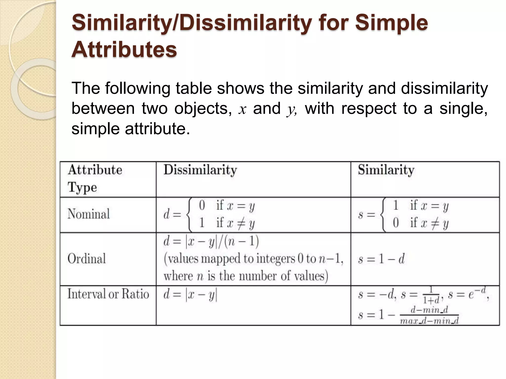
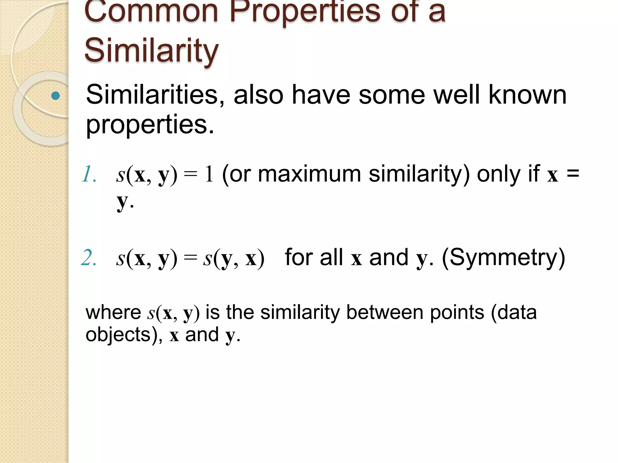
 Similarity measure
◦ Numerical measure of how alike two data objects
are.
◦ Is higher when objects are more alike.
◦ Often falls in the range [0,1]
 Dissimilarity measure
◦ Numerical measure of how different two data
objects are
◦ Lower when objects are more alike
◦ Minimum dissimilarity is often 0
◦ Upper limit varies
 Proximity refers to a similarity or dissimilarity

33. Similarity/Dissimilarity for Simple
Attributes
The following table shows the similarity and dissimilarity
between two objects, x and y, with respect to a single,
simple attribute.

34. Euclidean Distance
 Euclidean Distance
where n is the number of dimensions
(attributes) and xk and yk are, respectively,
the kth attributes (components) or data
objects x and y.
 Standardization is necessary, if scales differ.

35. Euclidean Distance
0
1
2
3
0 1 2 3 4 5 6
p1
p2
p3 p4
point x y
p1 0 2
p2 2 0
p3 3 1
p4 5 1
Distance Matrix
p1 p2 p3 p4
p1 0 2.828 3.162 5.099
p2 2.828 0 1.414 3.162
p3 3.162 1.414 0 2
p4 5.099 3.162 2 0

36. Minkowski Distance
 Minkowski Distance is a generalization of Euclidean
Distance
Where r is a parameter, n is the number of dimensions
(attributes) and xk and yk are, respectively, the kth
attributes (components) or data objects x and y.

37. Minkowski Distance: Examples
 r = 1. City block (Manhattan, taxicab, L1 norm)
distance.
◦ A common example of this is the Hamming distance,
which is just the number of bits that are different
between two binary vectors
 r = 2. Euclidean distance
 r  . “supremum” (Lmax norm, L norm) distance.
◦ This is the maximum difference between any component
of the vectors
 Do not confuse r with n, i.e., all these distances are
defined for all numbers of dimensions.

38. Minkowski Distance
Distance Matrix
point x y
p1 0 2
p2 2 0
p3 3 1
p4 5 1
L1 p1 p2 p3 p4
p1 0 4 4 6
p2 4 0 2 4
p3 4 2 0 2
p4 6 4 2 0
L2 p1 p2 p3 p4
p1 0 2.828 3.162 5.099
p2 2.828 0 1.414 3.162
p3 3.162 1.414 0 2
p4 5.099 3.162 2 0
L p1 p2 p3 p4
p1 0 2 3 5
p2 2 0 1 3
p3 3 1 0 2
p4 5 3 2 0

39. Mahalanobis Distance
For red points, the Euclidean distance is 14.7, Mahalanobis distance is 6.
 is the covariance matrix
𝐦𝐚𝐡𝐚𝐥𝐚𝐧𝐨𝐛𝐢𝐬 𝐱, 𝐲 = (𝐱 − 𝐲) 𝑇 Ʃ−1(𝐱 − 𝐲)

40. Mahalanobis Distance
Covariance
Matrix:







3.02.0
2.03.0
A: (0.5, 0.5)
B: (0, 1)
C: (1.5, 1.5)
Mahal(A,B) = 5
Mahal(A,C) = 4
B
A
C

41. Common Properties of a Distance
 Distances, such as the Euclidean distance,
have some well known properties.
1. d(x, y)  0 for all x and y and d(x, y) = 0 only if
x = y. (Positive definiteness)
2. d(x, y) = d(y, x) for all x and y. (Symmetry)
3. d(x, z)  d(x, y) + d(y, z) for all points x, y, and
z.
(Triangle Inequality)
where d(x, y) is the distance (dissimilarity) between points
(data objects), x and y.
 A distance that satisfies these properties is
a metric

42. Common Properties of a
Similarity
 Similarities, also have some well known
properties.
1. s(x, y) = 1 (or maximum similarity) only if x =
y.
2. s(x, y) = s(y, x) for all x and y. (Symmetry)
where s(x, y) is the similarity between points (data
objects), x and y.

43. Similarity Between Binary Vectors
 Common situation is that objects, p and q, have only
binary attributes
 Compute similarities using the following quantities
f01 = the number of attributes where p was 0 and q was 1
f10 = the number of attributes where p was 1 and q was 0
f00 = the number of attributes where p was 0 and q was 0
f11 = the number of attributes where p was 1 and q was 1
 Simple Matching and Jaccard Coefficients
SMC = number of matches / number of attributes
= (f11 + f00) / (f01 + f10 + f11 + f00)
J = number of 11 matches / number of non-zero attributes
= (f11) / (f01 + f10 + f11)

44. SMC versus Jaccard: Example
x = 1 0 0 0 0 0 0 0 0 0
y = 0 0 0 0 0 0 1 0 0 1
f01 = 2 (the number of attributes where p was 0 and q was 1)
f10 = 1 (the number of attributes where p was 1 and q was 0)
f00 = 7 (the number of attributes where p was 0 and q was 0)
f11 = 0 (the number of attributes where p was 1 and q was 1)
SMC = (f11 + f00) / (f01 + f10 + f11 + f00)
= (0+7) / (2+1+0+7) = 0.7
J = (f11) / (f01 + f10 + f11) = 0 / (2 + 1 + 0) = 0

45. Comparison of Proximity Measures
 Domain of application
◦ Similarity measures tend to be specific to the type of
attribute and data
◦ Record data, images, graphs, sequences, 3D-protein
structure, etc. tend to have different measures
 However, one can talk about various properties
that you would like a proximity measure to have
◦ Symmetry is a common one
◦ Tolerance to noise and outliers is another
◦ Ability to find more types of patterns?
◦ Many others possible
 The measure must be applicable to the data and
produce results that agree with domain knowledge

46. Information Based Measures
 Information theory is a well-developed
and fundamental disciple with broad
applications
 Some similarity measures are based on
information theory
◦ Mutual information in various versions
◦ Maximal Information Coefficient (MIC) and
related measures
◦ General and can handle non-linear
relationships
◦ Can be complicated and time intensive to
compute

47. Information and Probability
 Information relates to possible outcomes of an
event
◦ transmission of a message, flip of a coin, or
measurement of a piece of data
 The more certain an outcome, the less
information that it contains and vice-versa
◦ For example, if a coin has two heads, then an outcome
of heads provides no information
◦ More quantitatively, the information is related the
probability of an outcome
 The smaller the probability of an outcome, the more
information it provides and vice-versa
◦ Entropy is the commonly used measure

48. Density
 Measures the degree to which data objects are
close to each other in a specified area
 The notion of density is closely related to that of
proximity
 Concept of density is typically used for clustering
and anomaly detection
 Examples:
◦ Euclidean density
 Euclidean density = number of points per unit
volume
◦ Probability density
 Estimate what the distribution of the data looks like
◦ Graph-based density
 Connectivity

49. Euclidean Density: Grid-based
Approach
 Simplest approach is to divide region
into a number of rectangular cells of
equal volume and define density as #
of points the cell contains
Grid-based density. Counts for each cell.

50. Euclidean Density: Center-
Based
 Euclidean density is the number of
points within a specified radius of the
point
Illustration of center-based density.

51. Data Preprocessing
 Aggregation
 Sampling
 Dimensionality Reduction
 Feature subset selection
 Feature creation
 Discretization and Binarization
 Attribute Transformation

52. Aggregation
 Combining two or more attributes (or
objects) into a single attribute (or
object)
 Purpose
◦ Data reduction
 Reduce the number of attributes or objects
◦ Change of scale
 Cities aggregated into regions, states, countries,
etc.
 Days aggregated into weeks, months, or years
◦ More “stable” data
 Aggregated data tends to have less variability

53. Example: Precipitation in Australia
 This example is based on precipitation in Australia
from the period 1982 to 1993.
The next slide shows
◦ A histogram for the standard deviation of average
monthly precipitation for 3,030 0.5◦ by 0.5◦ grid cells in
Australia, and
◦ A histogram for the standard deviation of the average
yearly precipitation for the same locations.
 The average yearly precipitation has less
variability than the average monthly precipitation.
 All precipitation measurements (and their
standard deviations) are in centimeters.

54. Example: Precipitation in Australia …
Standard Deviation of Average
Monthly Precipitation
Standard Deviation of
Average Yearly Precipitation
Variation of Precipitation in Australia

55. Sampling
 Sampling is the main technique employed for
data reduction.
◦ It is often used for both the preliminary
investigation of the data and the final data
analysis.
 Statisticians often sample because obtaining
the entire set of data of interest is too
expensive or time consuming.
 Sampling is typically used in data mining
because processing the entire set of data of
interest is too expensive or time consuming.

56. Sampling …
 The key principle for effective sampling
is the following:
◦ Using a sample will work almost as well as
using the entire data set, if the sample is
representative
◦ A sample is representative if it has
approximately the same properties (of
interest) as the original set of data

57. Sample Size
8000 points 2000 Points 500 Points

58. Types of Sampling
 Simple Random Sampling
◦ There is an equal probability of selecting any
particular item
◦ Sampling without replacement
 As each item is selected, it is removed from the
population
◦ Sampling with replacement
 Objects are not removed from the population as they
are selected for the sample.
 In sampling with replacement, the same object can be
picked up more than once
 Stratified sampling
◦ Split the data into several partitions; then draw
random samples from each partition

59. Sample Size
 What sample size is necessary to get at least
one object from each of 10 equal-sized
groups.

60. Curse of Dimensionality
 When dimensionality
increases, data becomes
increasingly sparse in the
space that it occupies
 Definitions of density and
distance between points,
which are critical for
clustering and outlier
detection, become less
meaningful •Randomly generate 500 points
•Compute difference between max and
min distance between any pair of points

61. Dimensionality Reduction
 Purpose:
◦ Avoid curse of dimensionality
◦ Reduce amount of time and memory
required by data mining algorithms
◦ Allow data to be more easily visualized
◦ May help to eliminate irrelevant features
or reduce noise
 Techniques
◦ Principal Components Analysis (PCA)
◦ Singular Value Decomposition
◦ Others: supervised and non-linear

62. Dimensionality Reduction:
PCA
 Goal is to find a projection that
captures the largest amount of
variation in data
x2
x1
e

63. Dimensionality Reduction:
PCA

64. Feature Subset Selection
 Another way to reduce dimensionality of data
 Redundant features
◦ Duplicate much or all of the information contained in
one or more other attributes
◦ Example: purchase price of a product and the
amount of sales tax paid
 Irrelevant features
◦ Contain no information that is useful for the data
mining task at hand
◦ Example: students' ID is often irrelevant to the task
of predicting students' GPA
 Many techniques developed, especially for
classification

65. Feature Creation
 Create new attributes that can capture
the important information in a data set
much more efficiently than the original
attributes
 Three general methodologies:
◦ Feature extraction
 Example: extracting edges from images
◦ Feature construction
 Example: dividing mass by volume to get density
◦ Mapping data to new space
 Example: Fourier and wavelet analysis

66. Mapping Data to a New Space
Two Sine Waves + Noise Frequency
 Fourier and wavelet transform
Frequency

67. Discretization
 Discretization is the process of
converting a continuous attribute into an
ordinal attribute
◦ A potentially infinite number of values are
mapped into a small number of categories
◦ Discretization is commonly used in
classification
◦ Many classification algorithms work best if both
the independent and dependent variables have
only a few values
◦ We give an illustration of the usefulness of
discretization using the Iris data set

68. Iris Sample Data Set
 Iris Plant data set.
◦ Can be obtained from the UCI Machine Learning Repository
http://www.ics.uci.edu/~mlearn/MLRepository.html
◦ From the statistician Douglas Fisher
◦ Three flower types (classes):
 Setosa
 Versicolour
 Virginica
◦ Four (non-class) attributes
 Sepal width and length
 Petal width and length
Virginica. Robert H. Mohlenbrock. USDA NRCS.
1995. Northeast wetland flora: Field office guide to
plant species. Northeast National Technical Center,
Chester, PA. Courtesy of USDA NRCS Wetland
Science Institute.

69. Discretization: Iris Example
Petal width low or petal length low implies Setosa.
Petal width medium or petal length medium implies Versicolour.
Petal width high or petal length high implies Virginica.

70. Discretization: Iris Example …
 How can we tell what the best
discretization is?
◦ Unsupervised discretization: find breaks in the
data values
 Example:
Petal Length
◦ Supervised discretization: Use class labels to
find breaks
0 2 4 6 8
0
10
20
30
40
50
Petal Length
Counts

71. Discretization Without Using
Class Labels
Data consists of four groups of points and two outliers. Data is one-
dimensional, but a random y component is added to reduce overlap.

72. Discretization Without Using Class
Labels
Equal interval width approach used to obtain 4 values.

73. Discretization Without Using Clas
Labels
Equal frequency approach used to obtain 4 values.

74. Discretization Without Using Class
Labels
K-means approach to obtain 4 values.

75. Binarization
 Binarization maps a continuous or
categorical attribute into one or more binary
variables
 Typically used for association analysis
 Often convert a continuous attribute to a
categorical attribute and then convert a
categorical attribute to a set of binary
attributes
◦ Association analysis needs asymmetric binary
attributes
◦ Examples: eye color and height measured as
{low, medium, high}

76. Attribute Transformation
 An attribute transform is a function that maps
the entire set of values of a given attribute to
a new set of replacement values such that
each old value can be identified with one of
the new values
◦ Simple functions: xk, log(x), ex, |x|
◦ Normalization
 Refers to various techniques to adjust to differences
among attributes in terms of frequency of
occurrence, mean, variance, range
 Take out unwanted, common signal, e.g.,
seasonality
◦ In statistics, standardization refers to subtracting
off the means and dividing by the standard

77. Example: Sample Time Series of Plant Growth
Correlations between time series
Minneapolis
Minneapolis Atlanta Sao Paolo
Minneapolis 1.0000 0.7591 -0.7581
Atlanta 0.7591 1.0000 -0.5739
Sao Paolo -0.7581 -0.5739 1.0000
Correlations between time series
Net Primary
Production (NPP)
is a measure of
plant growth used
by ecosystem
scientists.