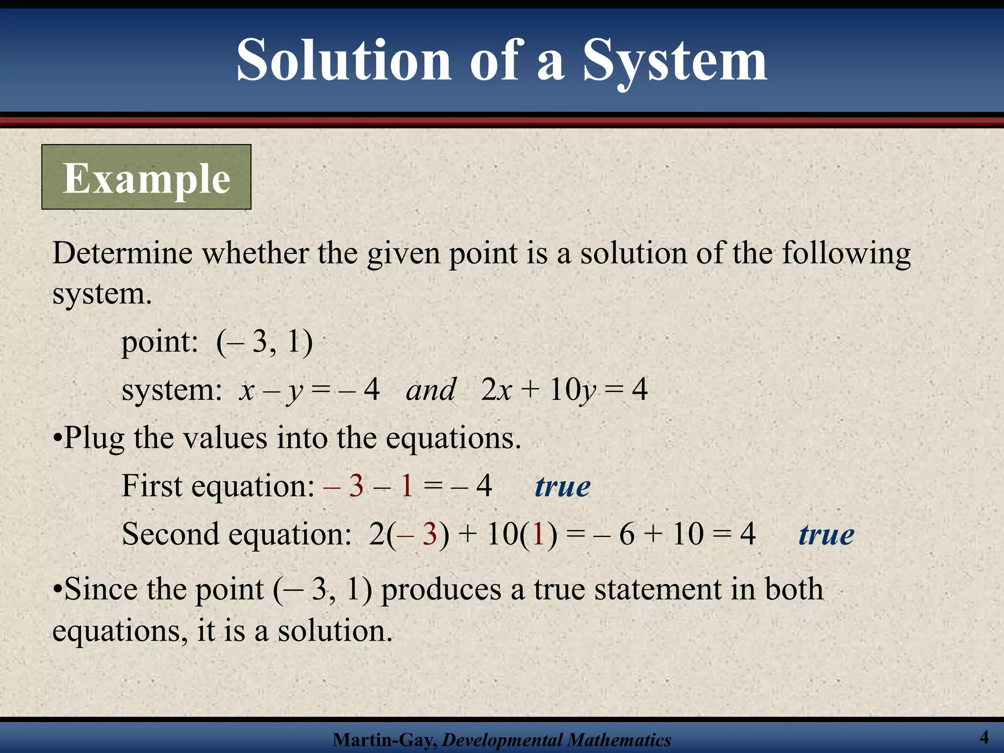
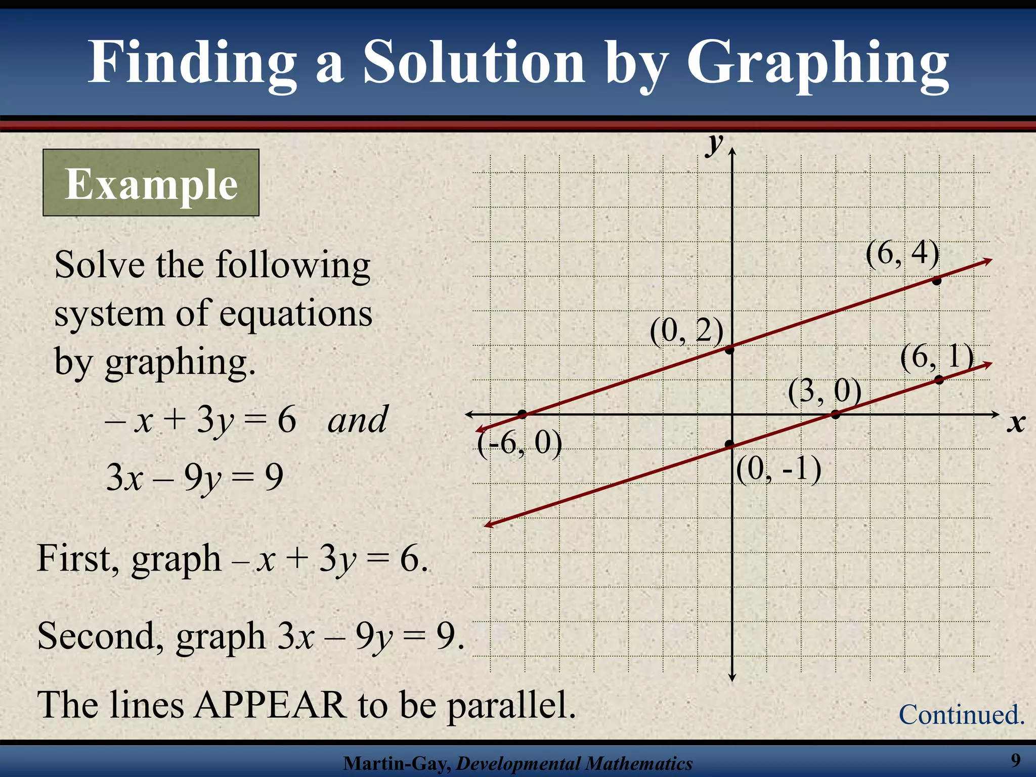
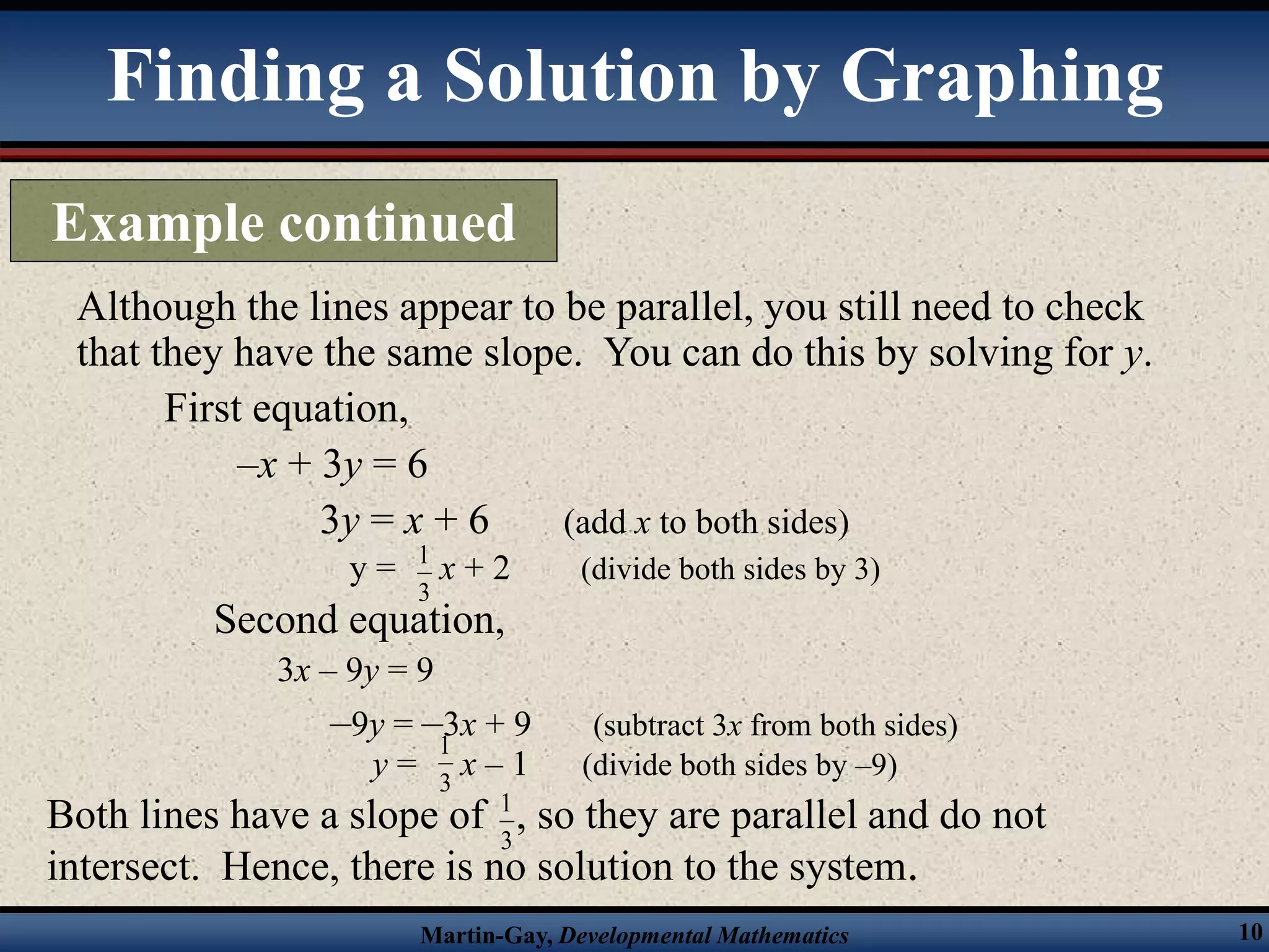
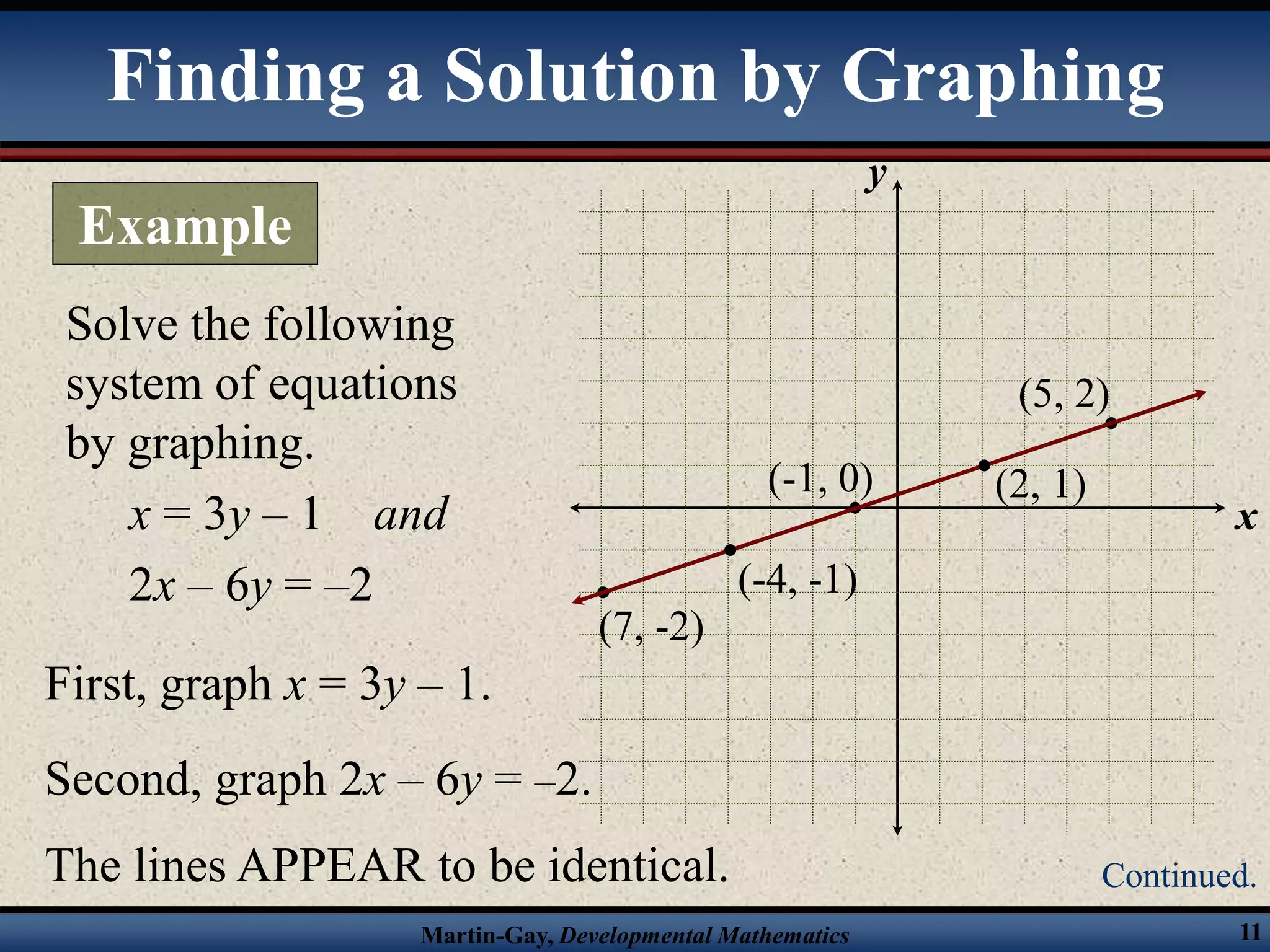
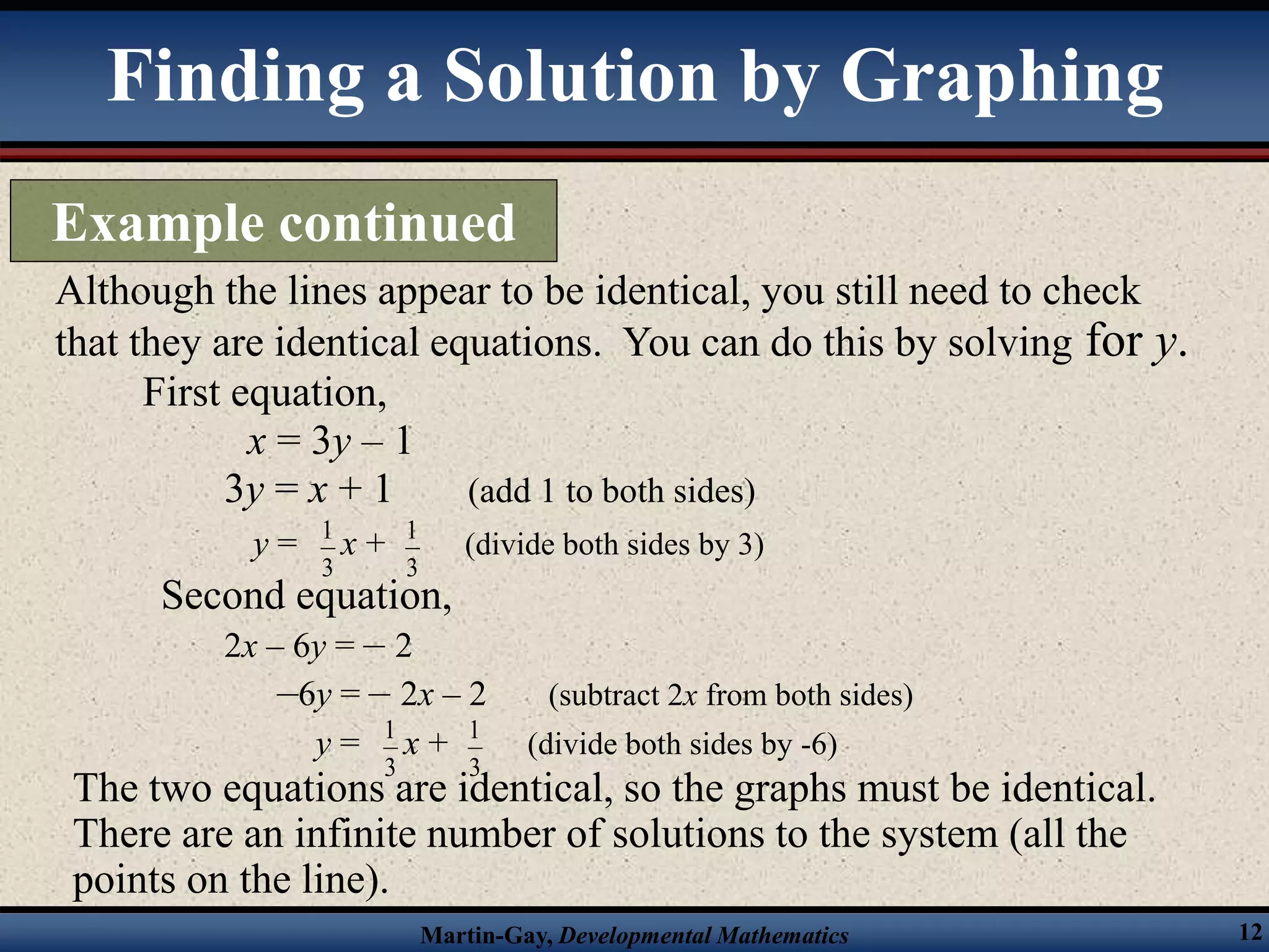
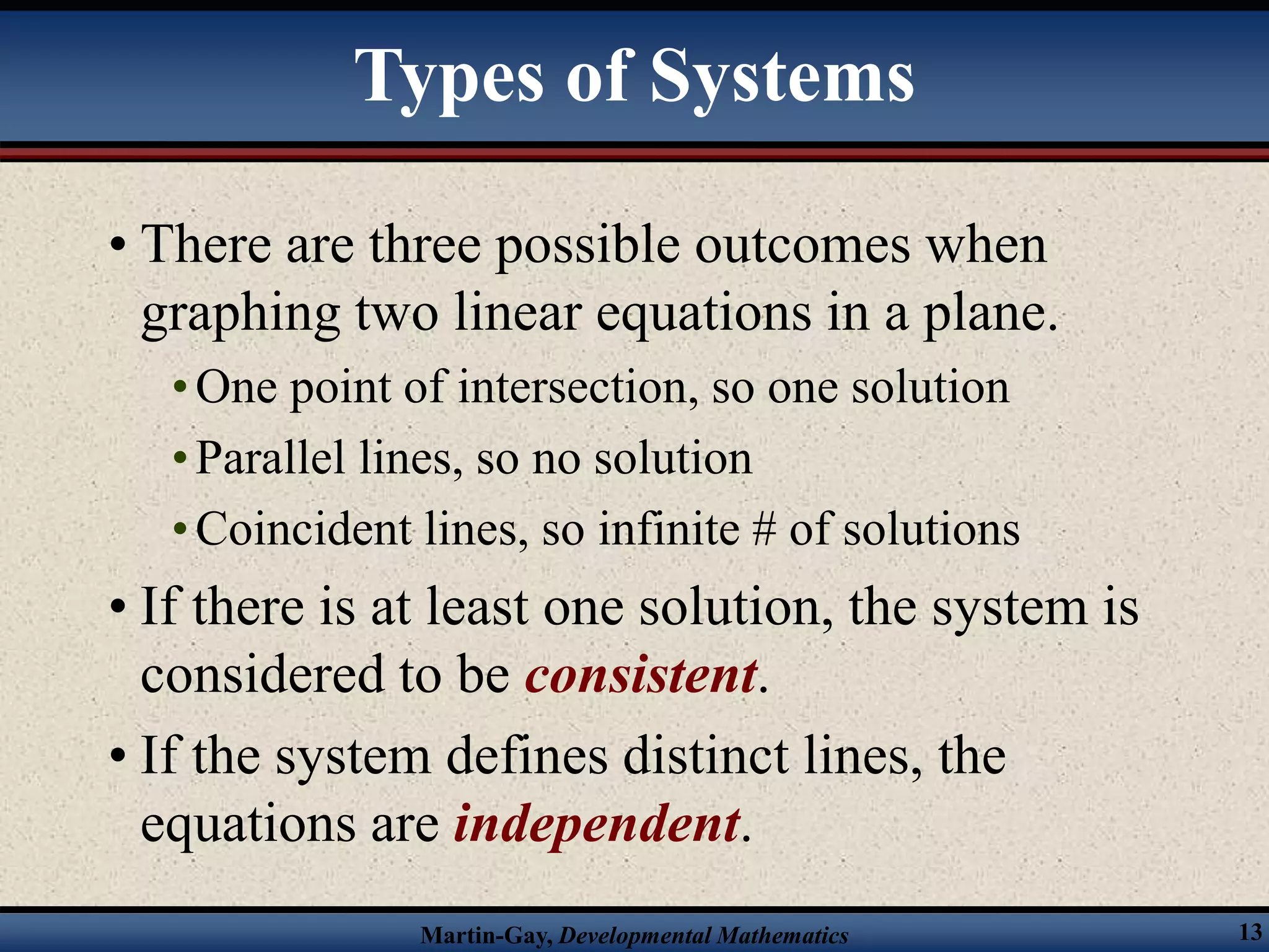
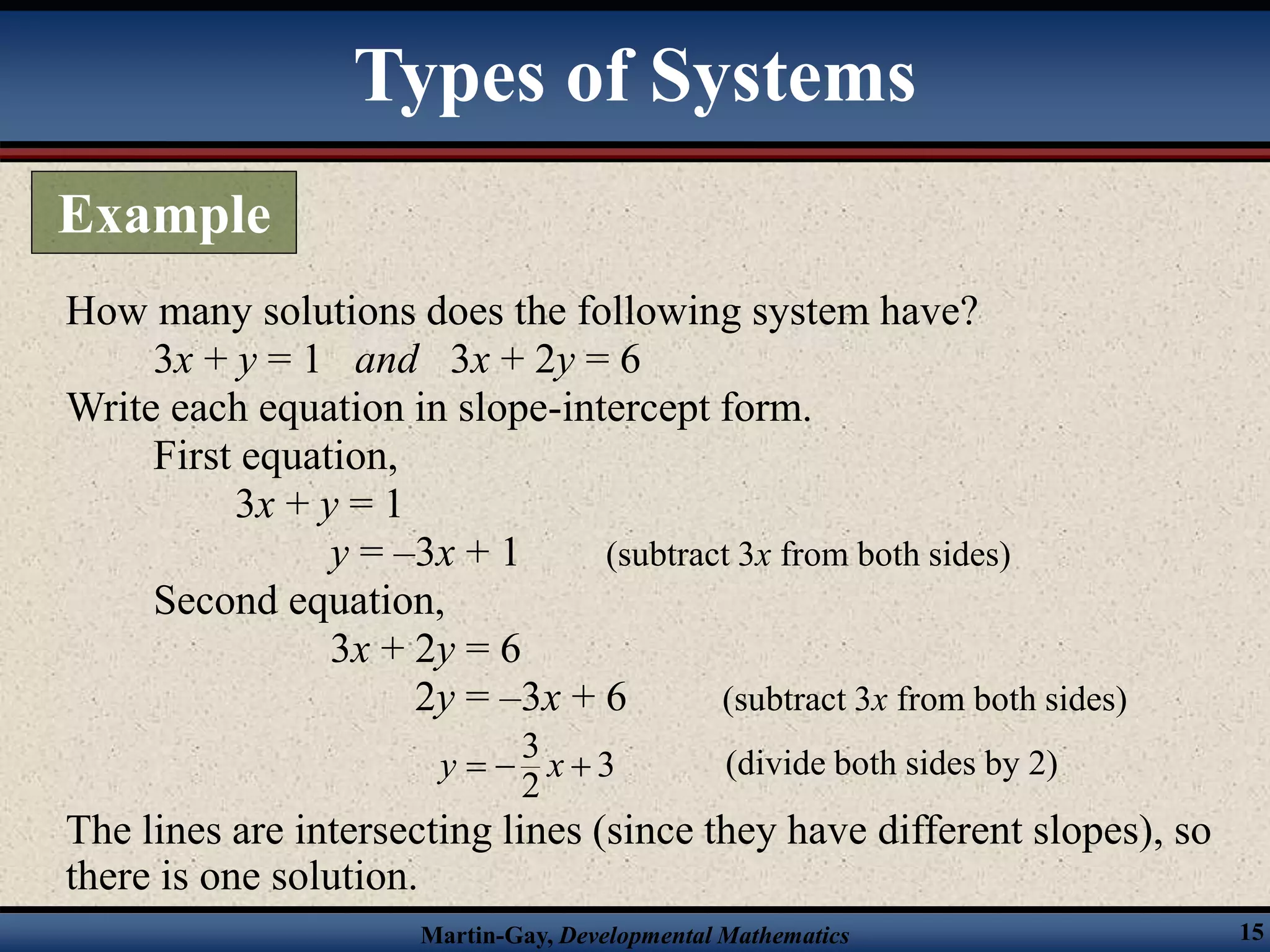
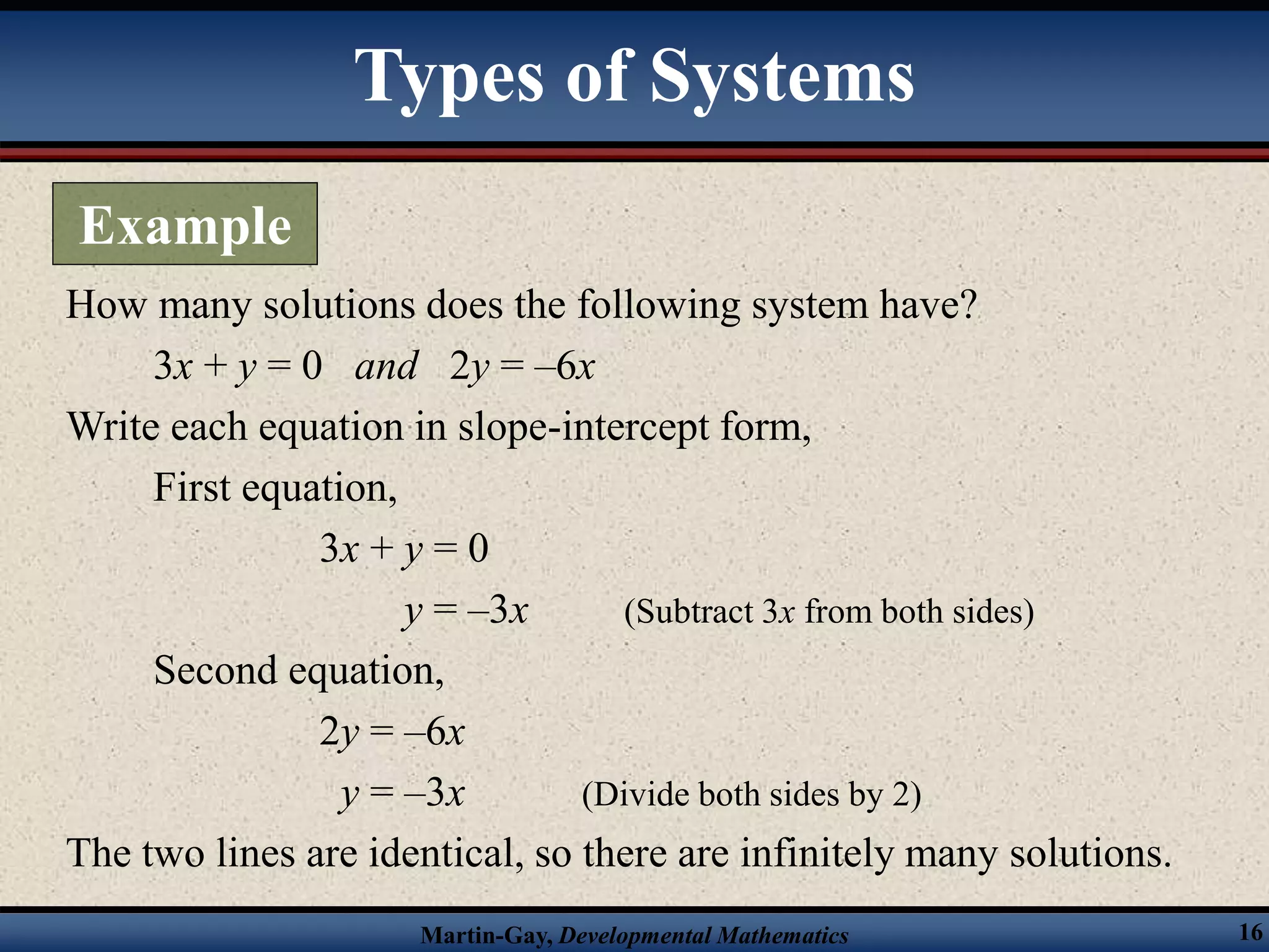
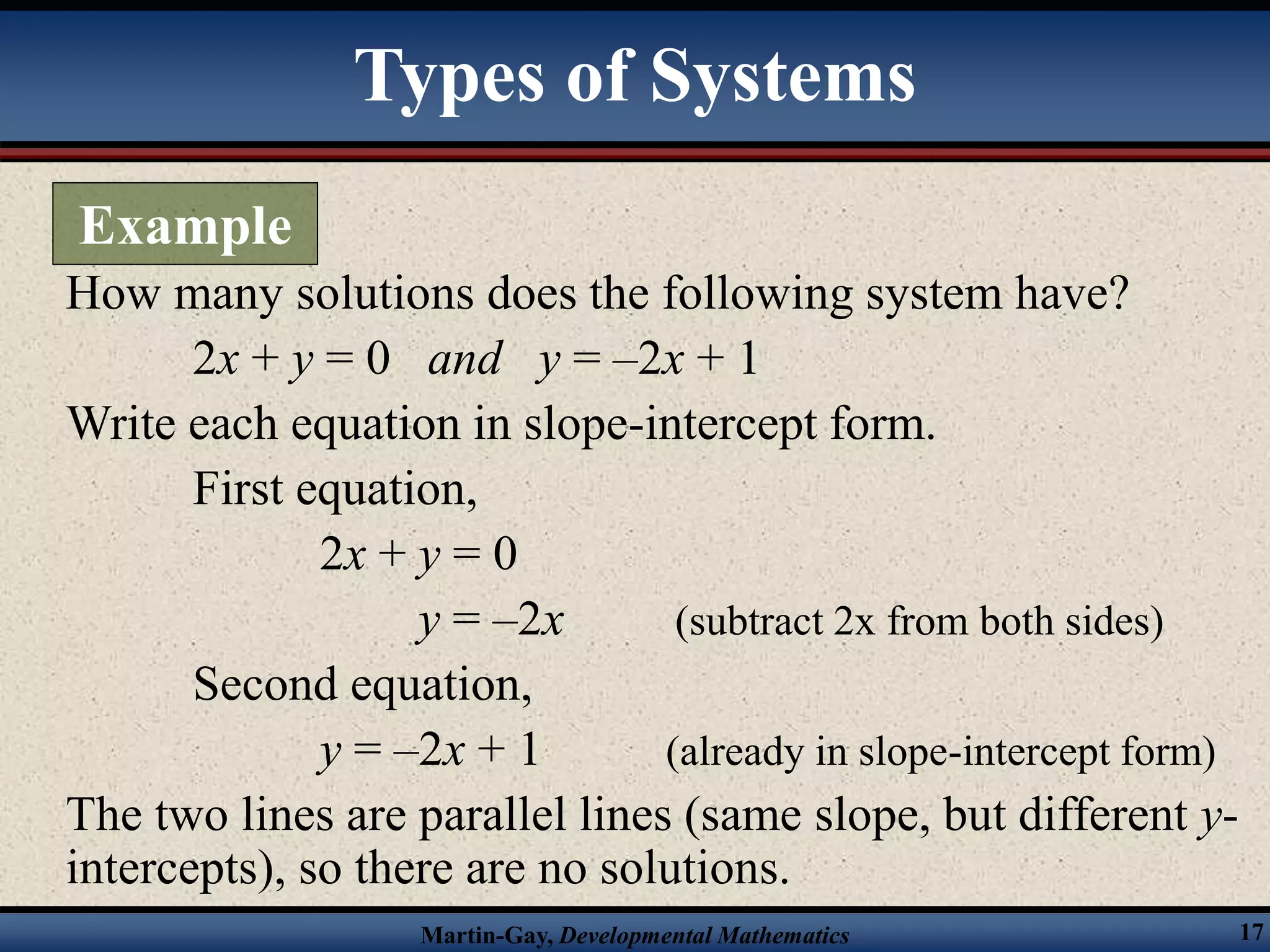
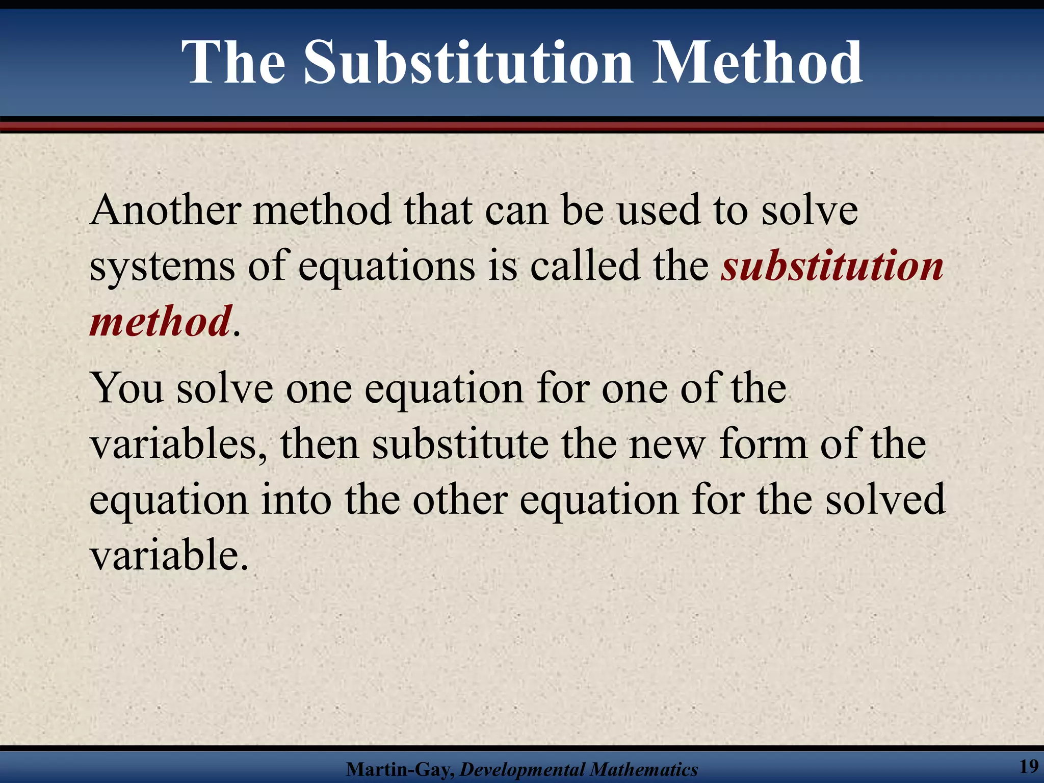
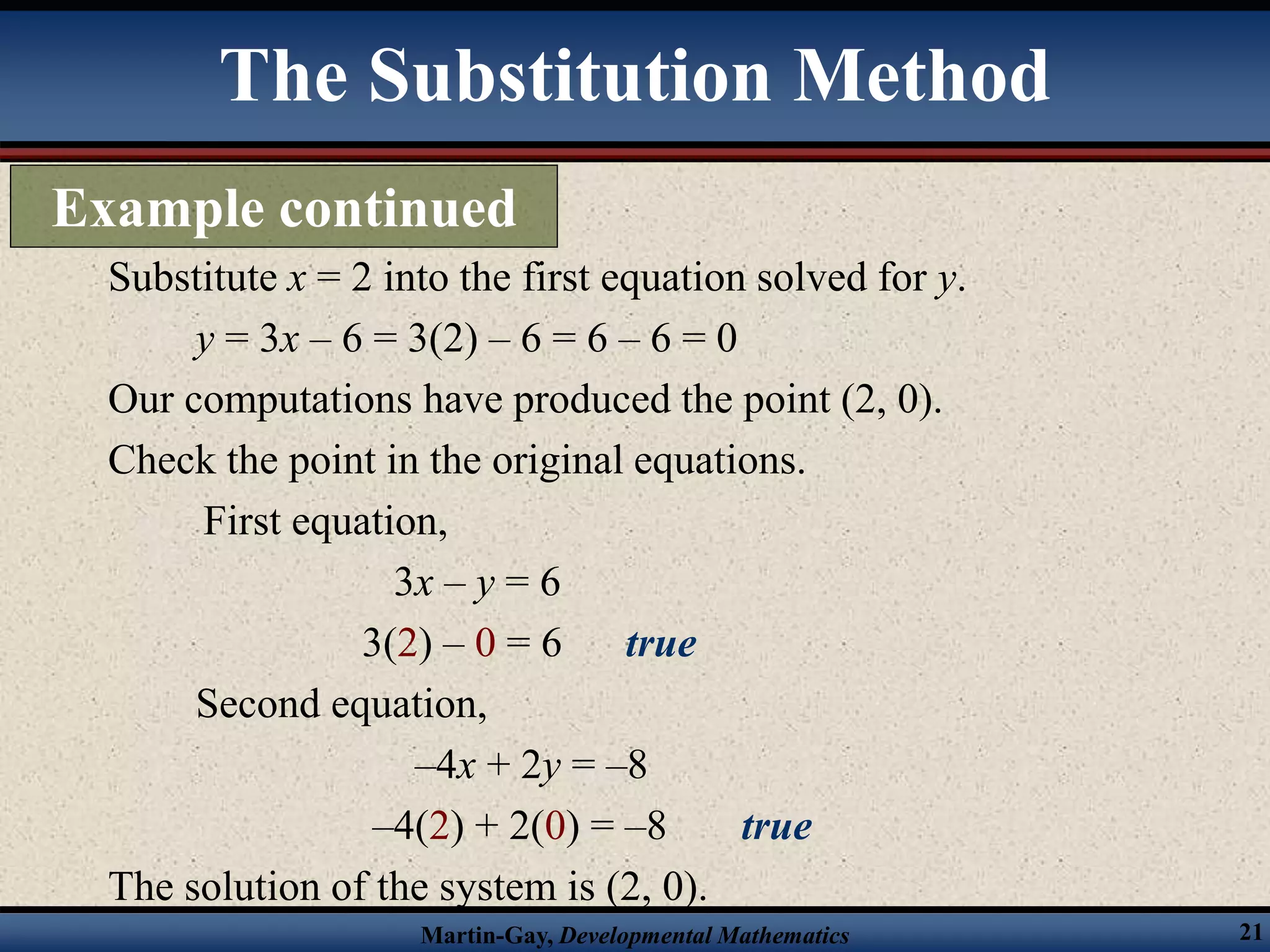
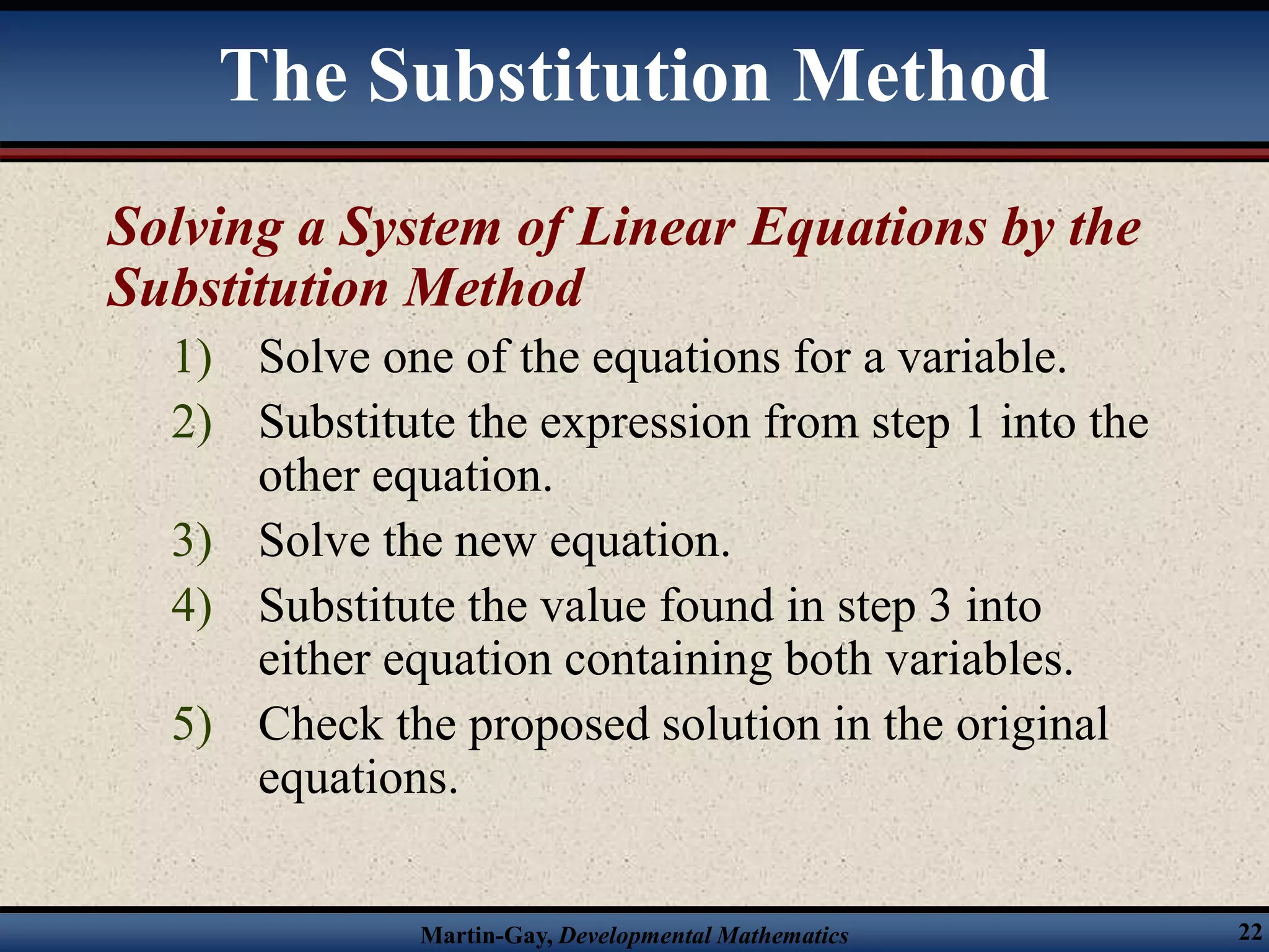
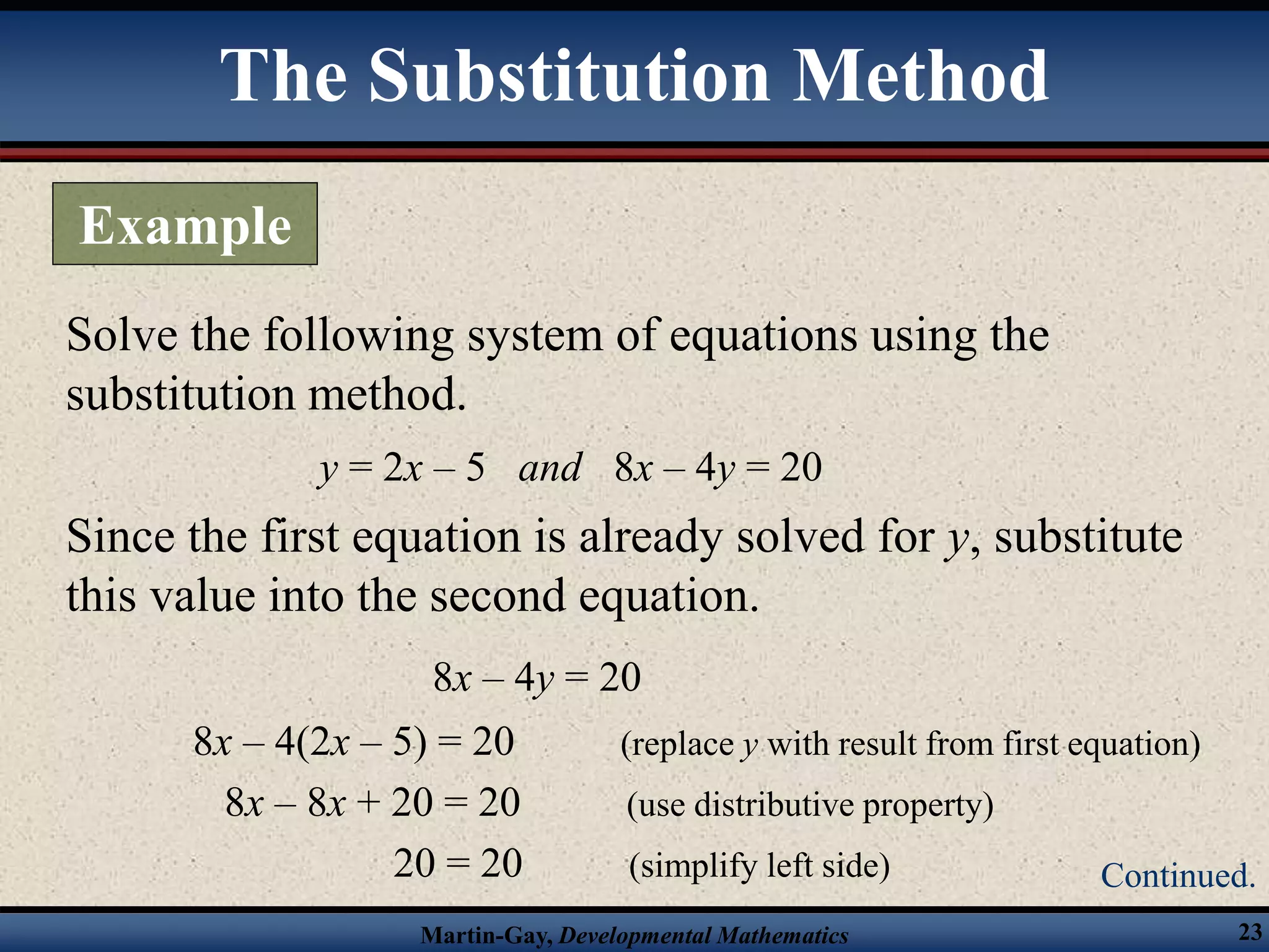
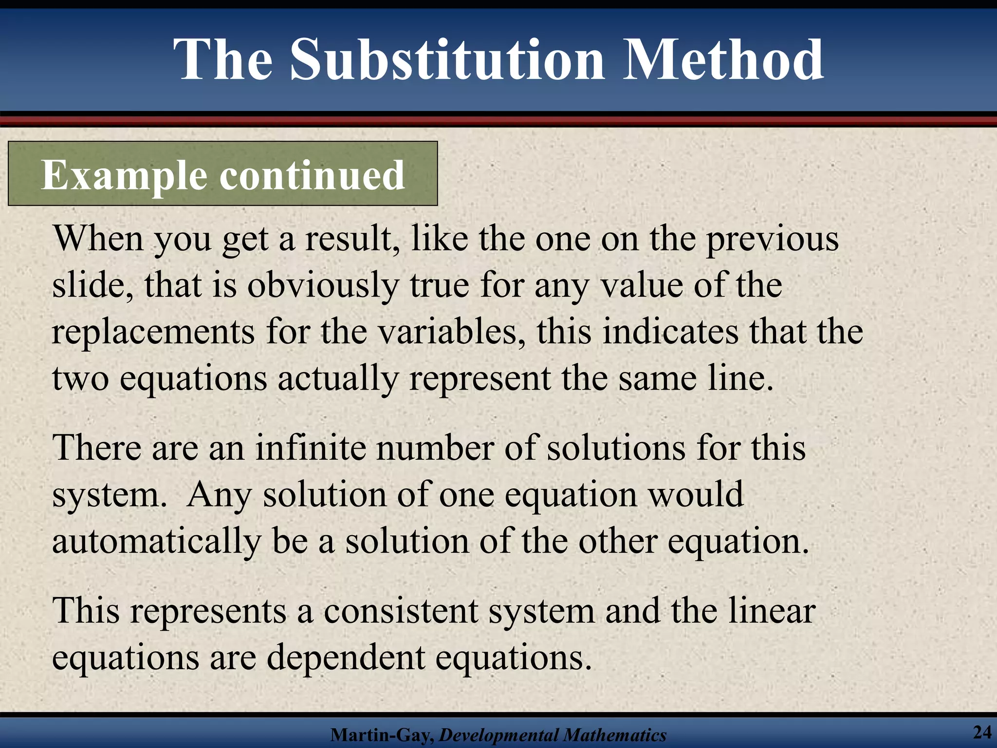
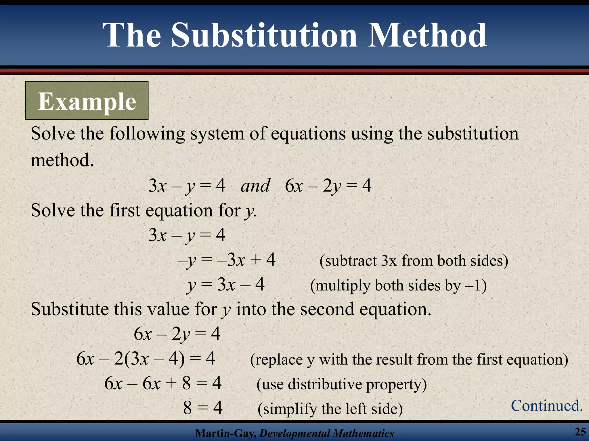
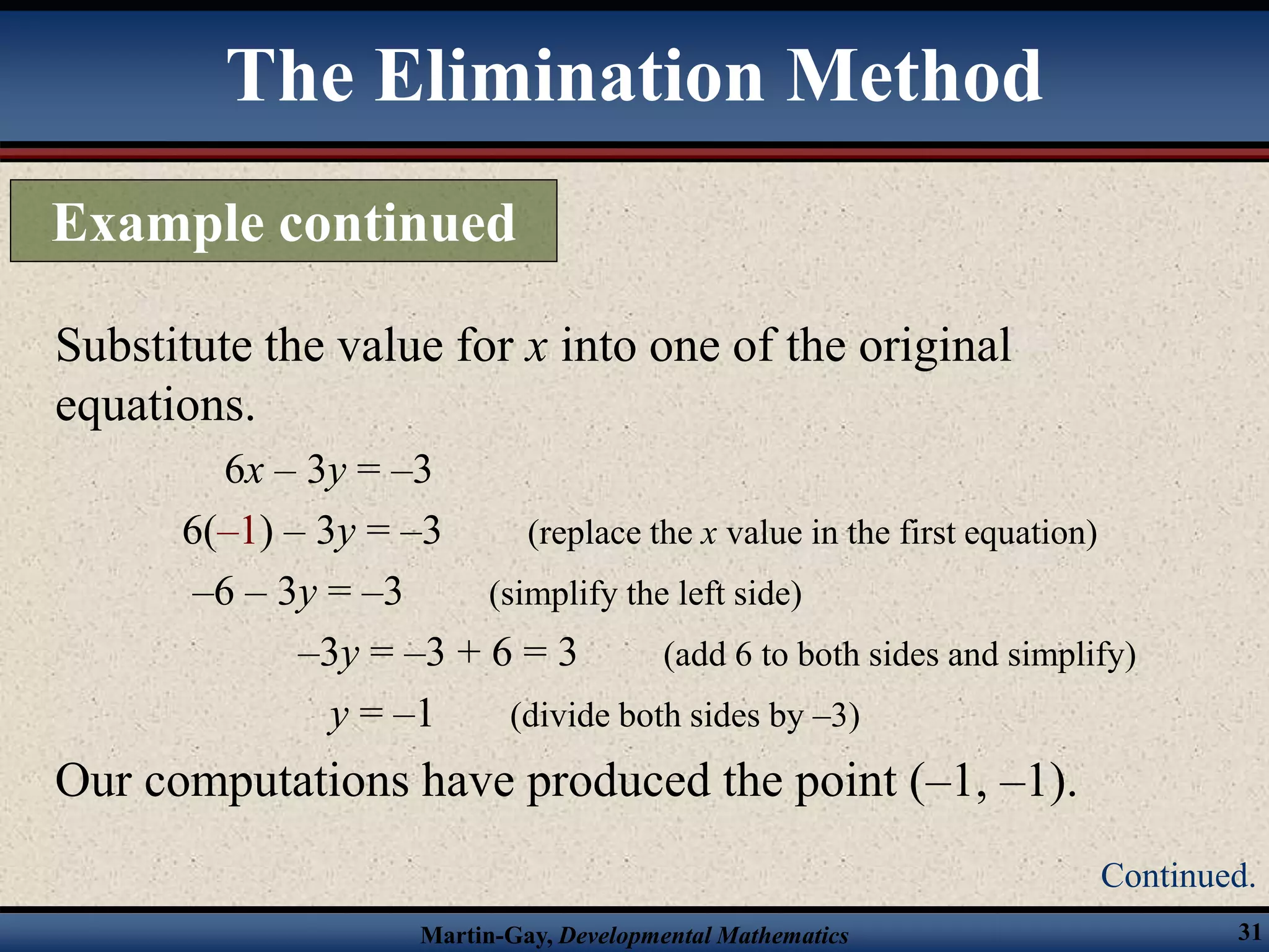
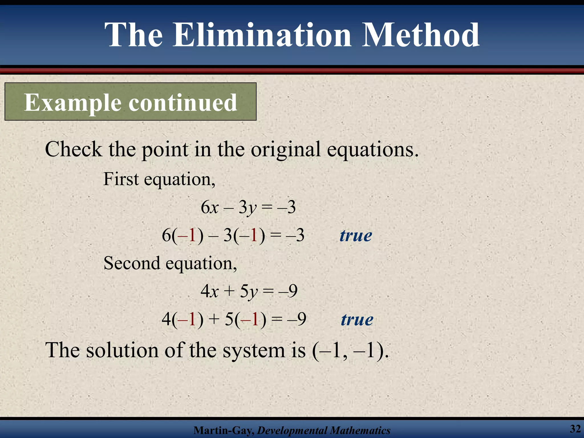
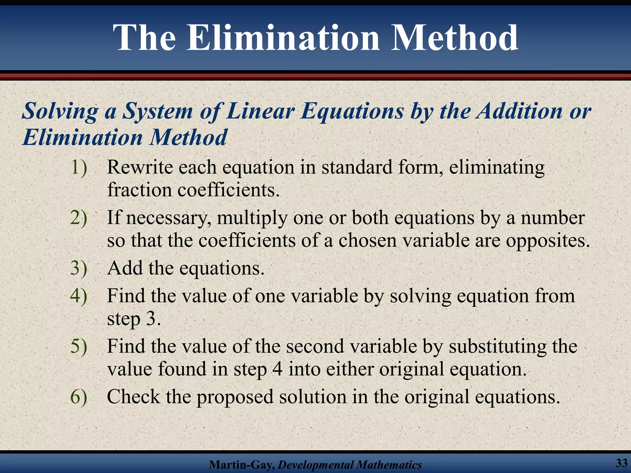
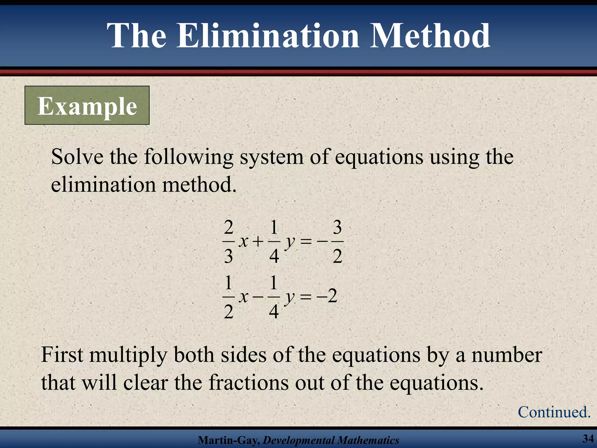
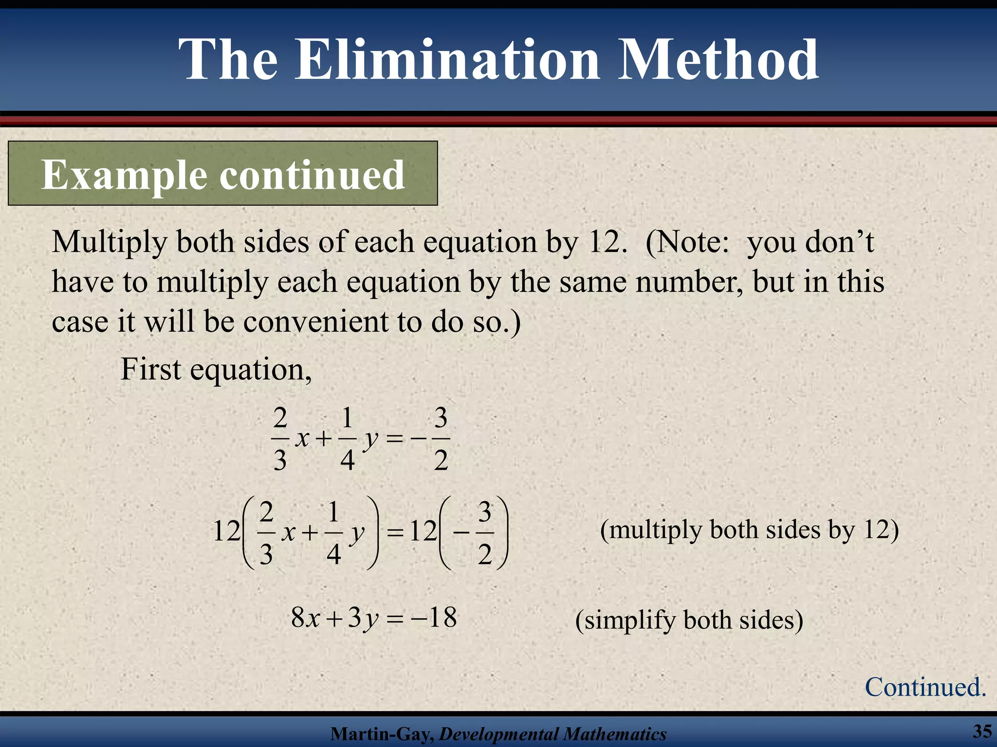
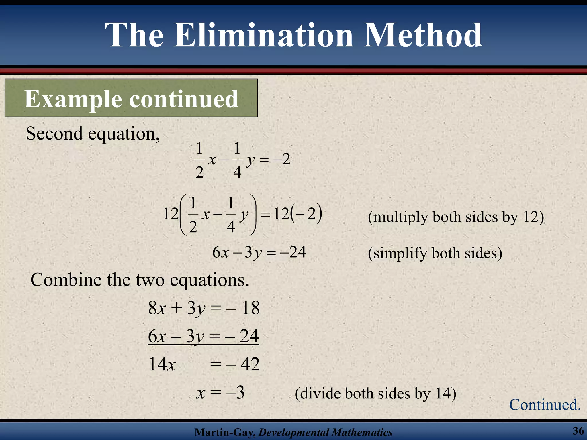
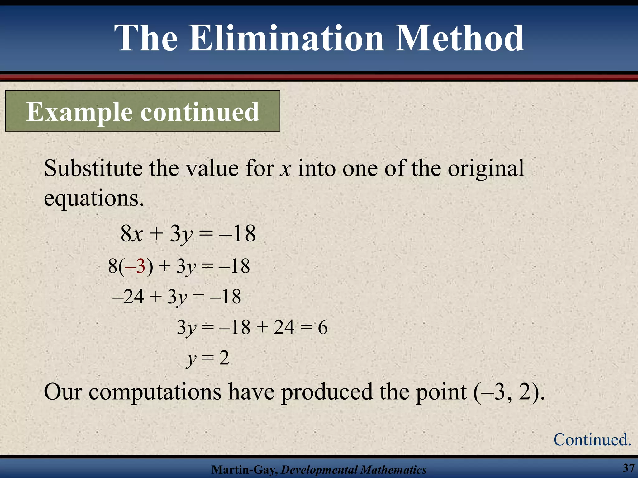
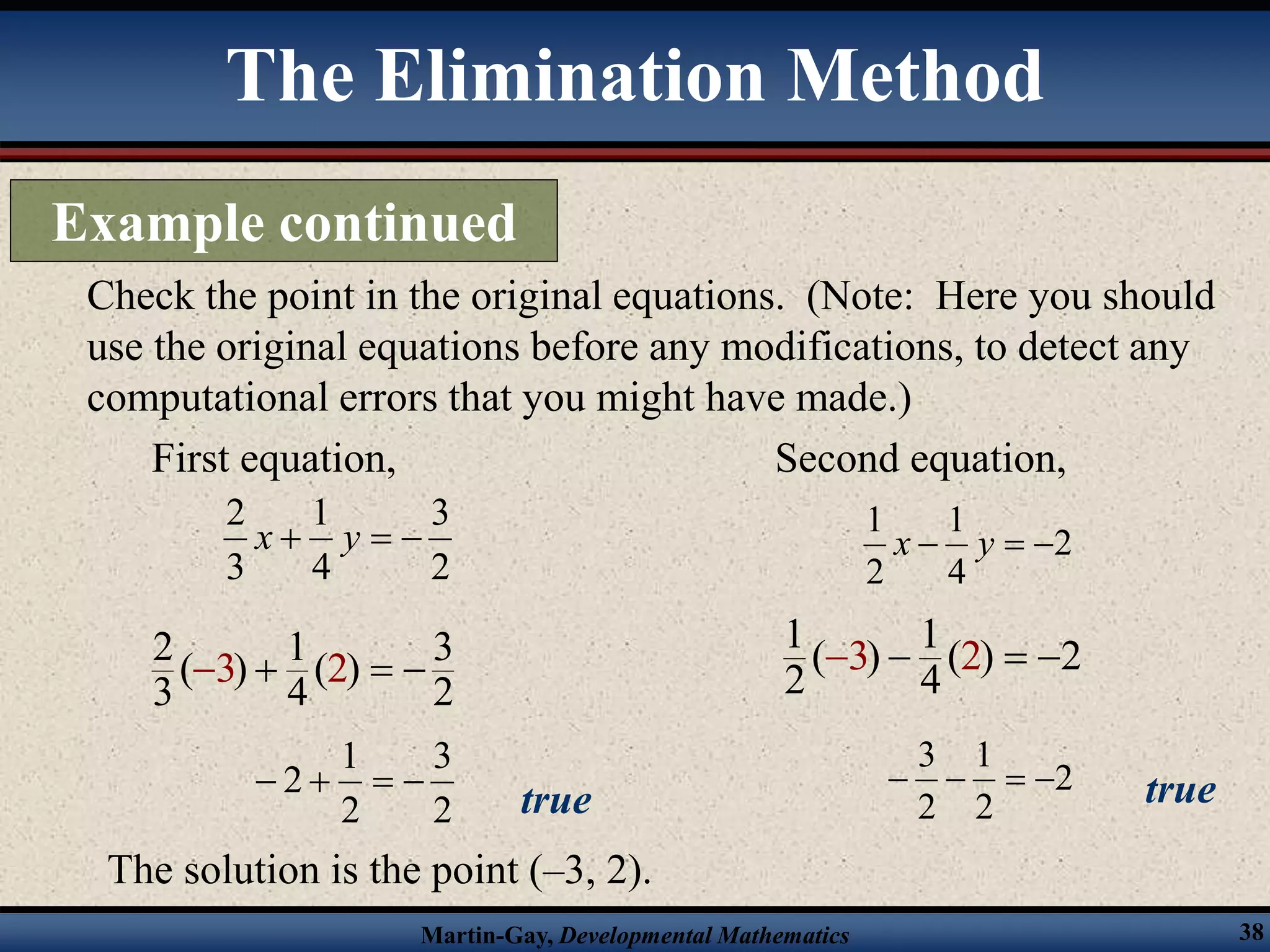
SlideShare a Scribd company logo
1 of 39
Chapter 3
Systems of
Equations
Solving Systems of Linear
Equations by Graphing
Martin-Gay, Developmental Mathematics 3
Systems of Linear Equations
A system of linear equations consists of two
or more linear equations.
This section focuses on only two equations at
a time.
The solution of a system of linear equations in
two variables is any ordered pair that solves
both of the linear equations.
Martin-Gay, Developmental Mathematics 4
Determine whether the given point is a solution of the following
system.
point: (– 3, 1)
system: x – y = – 4 and 2x + 10y = 4
•Plug the values into the equations.
First equation: – 3 – 1 = – 4 true
Second equation: 2(– 3) + 10(1) = – 6 + 10 = 4 true
•Since the point (– 3, 1) produces a true statement in both
equations, it is a solution.
Solution of a System
Example
Martin-Gay, Developmental Mathematics 5
Determine whether the given point is a solution of the following
system
point: (4, 2)
system: 2x – 5y = – 2 and 3x + 4y = 4
Plug the values into the equations
First equation: 2(4) – 5(2) = 8 – 10 = – 2 true
Second equation: 3(4) + 4(2) = 12 + 8 = 20  4 false
Since the point (4, 2) produces a true statement in only one
equation, it is NOT a solution.
Solution of a System
Example
Martin-Gay, Developmental Mathematics 6
• Since our chances of guessing the right coordinates
to try for a solution are not that high, we’ll be more
successful if we try a different technique.
• Since a solution of a system of equations is a
solution common to both equations, it would also
be a point common to the graphs of both equations.
• So to find the solution of a system of 2 linear
equations, graph the equations and see where the
lines intersect.
Finding a Solution by Graphing
Martin-Gay, Developmental Mathematics 7
Solve the following
system of equations
by graphing.
2x – y = 6 and
x + 3y = 10
x
y
First, graph 2x – y = 6.
(0, -6)
(3, 0)
(6, 6)
Second, graph x + 3y = 10.
(0, 10/3)
(-2, 4)
(-5, 5)
The lines APPEAR to intersect at (4, 2).
(4, 2)
Finding a Solution by Graphing
Example
Continued.
Martin-Gay, Developmental Mathematics 8
Although the solution to the system of equations appears
to be (4, 2), you still need to check the answer by
substituting x = 4 and y = 2 into the two equations.
First equation,
2(4) – 2 = 8 – 2 = 6 true
Second equation,
4 + 3(2) = 4 + 6 = 10 true
The point (4, 2) checks, so it is the solution of the
system.
Finding a Solution by Graphing
Example continued
Martin-Gay, Developmental Mathematics 9
Solve the following
system of equations
by graphing.
– x + 3y = 6 and
3x – 9y = 9
x
y
First, graph – x + 3y = 6.
(-6, 0)
(0, 2)
(6, 4)
Second, graph 3x – 9y = 9.
(0, -1)
(6, 1)
(3, 0)
The lines APPEAR to be parallel.
Finding a Solution by Graphing
Example
Continued.
Martin-Gay, Developmental Mathematics 10
Although the lines appear to be parallel, you still need to check
that they have the same slope. You can do this by solving for y.
First equation,
–x + 3y = 6
3y = x + 6 (add x to both sides)
3
1
y = x + 2 (divide both sides by 3)
Second equation,
3x – 9y = 9
–9y = –3x + 9 (subtract 3x from both sides)
3
1
y = x – 1 (divide both sides by –9)
3
1
Both lines have a slope of , so they are parallel and do not
intersect. Hence, there is no solution to the system.
Finding a Solution by Graphing
Example continued
Martin-Gay, Developmental Mathematics 11
Solve the following
system of equations
by graphing.
x = 3y – 1 and
2x – 6y = –2
x
y
First, graph x = 3y – 1.
(-1, 0)
(5, 2)
(7, -2)
Second, graph 2x – 6y = –2.
(-4, -1)
(2, 1)
The lines APPEAR to be identical.
Finding a Solution by Graphing
Example
Continued.
Martin-Gay, Developmental Mathematics 12
Although the lines appear to be identical, you still need to check
that they are identical equations. You can do this by solving for y.
First equation,
x = 3y – 1
3y = x + 1 (add 1 to both sides)
Second equation,
2x – 6y = – 2
–6y = – 2x – 2 (subtract 2x from both sides)
The two equations are identical, so the graphs must be identical.
There are an infinite number of solutions to the system (all the
points on the line).
3
1
y = x + (divide both sides by 3)
3
1
3
1
y = x + (divide both sides by -6)
3
1
Finding a Solution by Graphing
Example continued
Martin-Gay, Developmental Mathematics 13
• There are three possible outcomes when
graphing two linear equations in a plane.
•One point of intersection, so one solution
•Parallel lines, so no solution
•Coincident lines, so infinite # of solutions
• If there is at least one solution, the system is
considered to be consistent.
• If the system defines distinct lines, the
equations are independent.
Types of Systems
Martin-Gay, Developmental Mathematics 14
Change both linear equations into slope-
intercept form.
We can then easily determine if the lines
intersect, are parallel, or are the same line.
Types of Systems
Martin-Gay, Developmental Mathematics 15
How many solutions does the following system have?
3x + y = 1 and 3x + 2y = 6
Write each equation in slope-intercept form.
First equation,
3x + y = 1
y = –3x + 1 (subtract 3x from both sides)
Second equation,
3x + 2y = 6
2y = –3x + 6 (subtract 3x from both sides)
The lines are intersecting lines (since they have different slopes), so
there is one solution.
(divide both sides by 2)
3
3
2
y x
  
Types of Systems
Example
Martin-Gay, Developmental Mathematics 16
How many solutions does the following system have?
3x + y = 0 and 2y = –6x
Write each equation in slope-intercept form,
First equation,
3x + y = 0
y = –3x (Subtract 3x from both sides)
Second equation,
2y = –6x
y = –3x (Divide both sides by 2)
The two lines are identical, so there are infinitely many solutions.
Types of Systems
Example
Martin-Gay, Developmental Mathematics 17
How many solutions does the following system have?
2x + y = 0 and y = –2x + 1
Write each equation in slope-intercept form.
First equation,
2x + y = 0
y = –2x (subtract 2x from both sides)
Second equation,
y = –2x + 1 (already in slope-intercept form)
The two lines are parallel lines (same slope, but different y-
intercepts), so there are no solutions.
Types of Systems
Example
Solving Systems of Linear
Equations by Substitution
Martin-Gay, Developmental Mathematics 19
The Substitution Method
Another method that can be used to solve
systems of equations is called the substitution
method.
You solve one equation for one of the
variables, then substitute the new form of the
equation into the other equation for the solved
variable.
Martin-Gay, Developmental Mathematics 20
Solve the following system using the substitution method.
3x – y = 6 and – 4x + 2y = –8
Solving the first equation for y,
3x – y = 6
–y = –3x + 6 (subtract 3x from both sides)
y = 3x – 6 (divide both sides by – 1)
Substitute this value for y in the second equation.
–4x + 2y = –8
–4x + 2(3x – 6) = –8 (replace y with result from first equation)
–4x + 6x – 12 = –8 (use the distributive property)
2x – 12 = –8 (simplify the left side)
2x = 4 (add 12 to both sides)
x = 2 (divide both sides by 2)
The Substitution Method
Example
Continued.
Martin-Gay, Developmental Mathematics 21
Substitute x = 2 into the first equation solved for y.
y = 3x – 6 = 3(2) – 6 = 6 – 6 = 0
Our computations have produced the point (2, 0).
Check the point in the original equations.
First equation,
3x – y = 6
3(2) – 0 = 6 true
Second equation,
–4x + 2y = –8
–4(2) + 2(0) = –8 true
The solution of the system is (2, 0).
The Substitution Method
Example continued
Martin-Gay, Developmental Mathematics 22
Solving a System of Linear Equations by the
Substitution Method
1) Solve one of the equations for a variable.
2) Substitute the expression from step 1 into the
other equation.
3) Solve the new equation.
4) Substitute the value found in step 3 into
either equation containing both variables.
5) Check the proposed solution in the original
equations.
The Substitution Method
Martin-Gay, Developmental Mathematics 23
Solve the following system of equations using the
substitution method.
y = 2x – 5 and 8x – 4y = 20
Since the first equation is already solved for y, substitute
this value into the second equation.
8x – 4y = 20
8x – 4(2x – 5) = 20 (replace y with result from first equation)
8x – 8x + 20 = 20 (use distributive property)
20 = 20 (simplify left side)
The Substitution Method
Example
Continued.
Martin-Gay, Developmental Mathematics 24
When you get a result, like the one on the previous
slide, that is obviously true for any value of the
replacements for the variables, this indicates that the
two equations actually represent the same line.
There are an infinite number of solutions for this
system. Any solution of one equation would
automatically be a solution of the other equation.
This represents a consistent system and the linear
equations are dependent equations.
The Substitution Method
Example continued
Martin-Gay, Developmental Mathematics 25
Solve the following system of equations using the substitution
method.
3x – y = 4 and 6x – 2y = 4
Solve the first equation for y.
3x – y = 4
–y = –3x + 4 (subtract 3x from both sides)
y = 3x – 4 (multiply both sides by –1)
Substitute this value for y into the second equation.
6x – 2y = 4
6x – 2(3x – 4) = 4 (replace y with the result from the first equation)
6x – 6x + 8 = 4 (use distributive property)
8 = 4 (simplify the left side)
The Substitution Method
Example
Continued.
Martin-Gay, Developmental Mathematics 26
When you get a result, like the one on the previous
slide, that is never true for any value of the
replacements for the variables, this indicates that the
two equations actually are parallel and never
intersect.
There is no solution to this system.
This represents an inconsistent system, even though
the linear equations are independent.
The Substitution Method
Example continued
Solving Systems of Linear
Equations by Elimination
Martin-Gay, Developmental Mathematics 28
The Elimination Method
Another method that can be used to solve
systems of equations is called the addition,
arithmetic or elimination method.
You multiply both equations by numbers that
will allow you to combine the two equations
and eliminate one of the variables.
Martin-Gay, Developmental Mathematics 29
Solve the following system of equations using the elimination
method.
6x – 3y = –3 and 4x + 5y = –9
Multiply both sides of the first equation by 5 and the second
equation by 3.
First equation,
5(6x – 3y) = 5(–3)
30x – 15y = –15 (use the distributive property)
Second equation,
3(4x + 5y) = 3(–9)
12x + 15y = –27 (use the distributive property)
The Elimination Method
Example
Continued.
Martin-Gay, Developmental Mathematics 30
Combine the two resulting equations (eliminating the
variable y).
30x – 15y = –15
12x + 15y = –27
42x = –42
x = –1 (divide both sides by 42)
The Elimination Method
Example continued
Continued.
Martin-Gay, Developmental Mathematics 31
Substitute the value for x into one of the original
equations.
6x – 3y = –3
6(–1) – 3y = –3 (replace the x value in the first equation)
–6 – 3y = –3 (simplify the left side)
–3y = –3 + 6 = 3 (add 6 to both sides and simplify)
y = –1 (divide both sides by –3)
Our computations have produced the point (–1, –1).
The Elimination Method
Example continued
Continued.
Martin-Gay, Developmental Mathematics 32
Check the point in the original equations.
First equation,
6x – 3y = –3
6(–1) – 3(–1) = –3 true
Second equation,
4x + 5y = –9
4(–1) + 5(–1) = –9 true
The solution of the system is (–1, –1).
The Elimination Method
Example continued
Martin-Gay, Developmental Mathematics 33
Solving a System of Linear Equations by the Addition or
Elimination Method
1) Rewrite each equation in standard form, eliminating
fraction coefficients.
2) If necessary, multiply one or both equations by a number
so that the coefficients of a chosen variable are opposites.
3) Add the equations.
4) Find the value of one variable by solving equation from
step 3.
5) Find the value of the second variable by substituting the
value found in step 4 into either original equation.
6) Check the proposed solution in the original equations.
The Elimination Method
Martin-Gay, Developmental Mathematics 34
Solve the following system of equations using the
elimination method.
2
4
1
2
1
2
3
4
1
3
2






y
x
y
x
First multiply both sides of the equations by a number
that will clear the fractions out of the equations.
The Elimination Method
Example
Continued.
Martin-Gay, Developmental Mathematics 35
Multiply both sides of each equation by 12. (Note: you don’t
have to multiply each equation by the same number, but in this
case it will be convenient to do so.)
First equation,
2
3
4
1
3
2


 y
x















2
3
12
4
1
3
2
12 y
x (multiply both sides by 12)
18
3
8 

 y
x (simplify both sides)
The Elimination Method
Example continued
Continued.
Martin-Gay, Developmental Mathematics 36
Combine the two equations.
8x + 3y = – 18
6x – 3y = – 24
14x = – 42
x = –3 (divide both sides by 14)
Second equation,
2
4
1
2
1


 y
x
 
2
12
4
1
2
1
12 







 y
x (multiply both sides by 12)
(simplify both sides)
24
3
6 

 y
x
The Elimination Method
Example continued
Continued.
Martin-Gay, Developmental Mathematics 37
Substitute the value for x into one of the original
equations.
8x + 3y = –18
8(–3) + 3y = –18
–24 + 3y = –18
3y = –18 + 24 = 6
y = 2
Our computations have produced the point (–3, 2).
The Elimination Method
Example continued
Continued.
Martin-Gay, Developmental Mathematics 38
Check the point in the original equations. (Note: Here you should
use the original equations before any modifications, to detect any
computational errors that you might have made.)
First equation,
2
3
4
1
3
2


 y
x
2 1 3
( ) ( )
3 4 2
3 2
  

2
3
2
1
2 



true
Second equation,
2
4
1
2
1


 y
x
1 1
( ) ( ) 2
2 4
3 2
  

2
2
1
2
3



 true
The solution is the point (–3, 2).
The Elimination Method
Example continued
Martin-Gay, Developmental Mathematics 39
In a similar fashion to what you found in the
last section, use of the elimination method to
combine two equations might lead you to
results like . . .
5 = 5 (which is always true, thus indicating that
there are infinitely many solutions, since the two
equations represent the same line), or
0 = 6 (which is never true, thus indicating that
there are no solutions, since the two equations
represent parallel lines).
Special Cases

More Related Content

What's hot

Introduction to slope presentation
Introduction to slope presentationIntroduction to slope presentation
Introduction to slope presentation
skellyreyes
 
Solving systems of equations in 3 variables
Solving systems of equations in 3 variablesSolving systems of equations in 3 variables
Solving systems of equations in 3 variables
Jessica Garcia
 
Ultimate guide to linear inequalities
Ultimate guide to linear inequalitiesUltimate guide to linear inequalities
Ultimate guide to linear inequalities
khyps13
 
7.6 solving logarithmic equations
7.6 solving logarithmic equations7.6 solving logarithmic equations
7.6 solving logarithmic equations
swartzje
 
Linear Equations Ppt
Linear Equations PptLinear Equations Ppt
Linear Equations Ppt
Scott R
 

What's hot (20)

Systems of Linear Algebra
Systems of Linear AlgebraSystems of Linear Algebra
Systems of Linear Algebra
 
Remainder and Factor Theorem
Remainder and Factor TheoremRemainder and Factor Theorem
Remainder and Factor Theorem
 
Tutorials: Solving Two-Step Equations
Tutorials: Solving Two-Step EquationsTutorials: Solving Two-Step Equations
Tutorials: Solving Two-Step Equations
 
Introduction to slope presentation
Introduction to slope presentationIntroduction to slope presentation
Introduction to slope presentation
 
Graphing linear equations
Graphing linear equationsGraphing linear equations
Graphing linear equations
 
11.2 graphing linear equations in two variables
11.2 graphing linear equations in two variables11.2 graphing linear equations in two variables
11.2 graphing linear equations in two variables
 
Exponents and Polynomials
Exponents and Polynomials Exponents and Polynomials
Exponents and Polynomials
 
Solving systems of equations in 3 variables
Solving systems of equations in 3 variablesSolving systems of equations in 3 variables
Solving systems of equations in 3 variables
 
PAIR OF LINEAR EQUATION IN TWO VARIABLE
PAIR OF LINEAR EQUATION IN TWO VARIABLEPAIR OF LINEAR EQUATION IN TWO VARIABLE
PAIR OF LINEAR EQUATION IN TWO VARIABLE
 
Factoring general trinomials
Factoring general trinomialsFactoring general trinomials
Factoring general trinomials
 
Ultimate guide to linear inequalities
Ultimate guide to linear inequalitiesUltimate guide to linear inequalities
Ultimate guide to linear inequalities
 
Section 8: Symmetric Groups
Section 8: Symmetric GroupsSection 8: Symmetric Groups
Section 8: Symmetric Groups
 
7.6 solving logarithmic equations
7.6 solving logarithmic equations7.6 solving logarithmic equations
7.6 solving logarithmic equations
 
Factoring Quadratic Trinomials
Factoring Quadratic TrinomialsFactoring Quadratic Trinomials
Factoring Quadratic Trinomials
 
arithmetic means
 arithmetic means arithmetic means
arithmetic means
 
Solve By Elimination
Solve By EliminationSolve By Elimination
Solve By Elimination
 
Linear Equations Ppt
Linear Equations PptLinear Equations Ppt
Linear Equations Ppt
 
Linear equations and thier use in practical life
Linear equations and thier use in practical lifeLinear equations and thier use in practical life
Linear equations and thier use in practical life
 
GRADE 10 ARITHMETIC.pptx
GRADE 10 ARITHMETIC.pptxGRADE 10 ARITHMETIC.pptx
GRADE 10 ARITHMETIC.pptx
 
Translating Mathematical Phrases to rational algebraic expressions 200827031831
Translating Mathematical Phrases to rational algebraic expressions 200827031831Translating Mathematical Phrases to rational algebraic expressions 200827031831
Translating Mathematical Phrases to rational algebraic expressions 200827031831
 

Similar to Linear Algebra - systems of equations (week 1).ppt

Systems of Linear Equations
Systems of Linear EquationsSystems of Linear Equations
Systems of Linear Equations
alrosiemae
 
Linear equations rev
Linear equations revLinear equations rev
Linear equations rev
Yash Jain
 
Linear equations rev - copy
Linear equations rev - copyLinear equations rev - copy
Linear equations rev - copy
Yash Jain
 
Pair of linear equations
Pair of linear equationsPair of linear equations
Pair of linear equations
Yash Jain
 
Solving systems of Linear Equations
Solving systems of Linear EquationsSolving systems of Linear Equations
Solving systems of Linear Equations
swartzje
 
February 13, 2015
February 13, 2015February 13, 2015
February 13, 2015
khyps13
 
February 18, 2015
February 18, 2015February 18, 2015
February 18, 2015
khyps13
 
January18
January18January18
January18
khyps13
 
Final presentation
Final presentationFinal presentation
Final presentation
paezp
 

Similar to Linear Algebra - systems of equations (week 1).ppt (20)

Linear equations
Linear equationsLinear equations
Linear equations
 
7.2
7.27.2
7.2
 
Systems of Linear Equations
Systems of Linear EquationsSystems of Linear Equations
Systems of Linear Equations
 
Linear Equations
Linear Equations Linear Equations
Linear Equations
 
Linear equations rev
Linear equations revLinear equations rev
Linear equations rev
 
Linear equations rev - copy
Linear equations rev - copyLinear equations rev - copy
Linear equations rev - copy
 
Pair of linear equations
Pair of linear equationsPair of linear equations
Pair of linear equations
 
Systems of linear equations
Systems of linear equationsSystems of linear equations
Systems of linear equations
 
Solving systems of Linear Equations
Solving systems of Linear EquationsSolving systems of Linear Equations
Solving systems of Linear Equations
 
February 13, 2015
February 13, 2015February 13, 2015
February 13, 2015
 
M1 L5 Remediation Notes
M1 L5 Remediation NotesM1 L5 Remediation Notes
M1 L5 Remediation Notes
 
February 18, 2015
February 18, 2015February 18, 2015
February 18, 2015
 
January18
January18January18
January18
 
Linear equations
Linear equationsLinear equations
Linear equations
 
Solving Systems of Linear Equations by Graphing
Solving  Systems of Linear Equations by Graphing Solving  Systems of Linear Equations by Graphing
Solving Systems of Linear Equations by Graphing
 
Linear equation in 2 variables
Linear equation in 2 variablesLinear equation in 2 variables
Linear equation in 2 variables
 
LecturePresentation.pptx
LecturePresentation.pptxLecturePresentation.pptx
LecturePresentation.pptx
 
Mathematics 8 Systems of Linear Inequalities
Mathematics 8 Systems of Linear InequalitiesMathematics 8 Systems of Linear Inequalities
Mathematics 8 Systems of Linear Inequalities
 
Final presentation
Final presentationFinal presentation
Final presentation
 
Linear equation in two variables
Linear equation in two variablesLinear equation in two variables
Linear equation in two variables
 

Recently uploaded

The basics of sentences session 3pptx.pptx
The basics of sentences session 3pptx.pptxThe basics of sentences session 3pptx.pptx
The basics of sentences session 3pptx.pptx
heathfieldcps1
 

Recently uploaded (20)

Sensory_Experience_and_Emotional_Resonance_in_Gabriel_Okaras_The_Piano_and_Th...
Sensory_Experience_and_Emotional_Resonance_in_Gabriel_Okaras_The_Piano_and_Th...Sensory_Experience_and_Emotional_Resonance_in_Gabriel_Okaras_The_Piano_and_Th...
Sensory_Experience_and_Emotional_Resonance_in_Gabriel_Okaras_The_Piano_and_Th...
 
Jamworks pilot and AI at Jisc (20/03/2024)
Jamworks pilot and AI at Jisc (20/03/2024)Jamworks pilot and AI at Jisc (20/03/2024)
Jamworks pilot and AI at Jisc (20/03/2024)
 
dusjagr & nano talk on open tools for agriculture research and learning
dusjagr & nano talk on open tools for agriculture research and learningdusjagr & nano talk on open tools for agriculture research and learning
dusjagr & nano talk on open tools for agriculture research and learning
 
On National Teacher Day, meet the 2024-25 Kenan Fellows
On National Teacher Day, meet the 2024-25 Kenan FellowsOn National Teacher Day, meet the 2024-25 Kenan Fellows
On National Teacher Day, meet the 2024-25 Kenan Fellows
 
80 ĐỀ THI THỬ TUYỂN SINH TIẾNG ANH VÀO 10 SỞ GD – ĐT THÀNH PHỐ HỒ CHÍ MINH NĂ...
80 ĐỀ THI THỬ TUYỂN SINH TIẾNG ANH VÀO 10 SỞ GD – ĐT THÀNH PHỐ HỒ CHÍ MINH NĂ...80 ĐỀ THI THỬ TUYỂN SINH TIẾNG ANH VÀO 10 SỞ GD – ĐT THÀNH PHỐ HỒ CHÍ MINH NĂ...
80 ĐỀ THI THỬ TUYỂN SINH TIẾNG ANH VÀO 10 SỞ GD – ĐT THÀNH PHỐ HỒ CHÍ MINH NĂ...
 
Details on CBSE Compartment Exam.pptx1111
Details on CBSE Compartment Exam.pptx1111Details on CBSE Compartment Exam.pptx1111
Details on CBSE Compartment Exam.pptx1111
 
How to setup Pycharm environment for Odoo 17.pptx
How to setup Pycharm environment for Odoo 17.pptxHow to setup Pycharm environment for Odoo 17.pptx
How to setup Pycharm environment for Odoo 17.pptx
 
VAMOS CUIDAR DO NOSSO PLANETA! .
VAMOS CUIDAR DO NOSSO PLANETA!                    .VAMOS CUIDAR DO NOSSO PLANETA!                    .
VAMOS CUIDAR DO NOSSO PLANETA! .
 
FSB Advising Checklist - Orientation 2024
FSB Advising Checklist - Orientation 2024FSB Advising Checklist - Orientation 2024
FSB Advising Checklist - Orientation 2024
 
How to Manage Call for Tendor in Odoo 17
How to Manage Call for Tendor in Odoo 17How to Manage Call for Tendor in Odoo 17
How to Manage Call for Tendor in Odoo 17
 
UGC NET Paper 1 Unit 7 DATA INTERPRETATION.pdf
UGC NET Paper 1 Unit 7 DATA INTERPRETATION.pdfUGC NET Paper 1 Unit 7 DATA INTERPRETATION.pdf
UGC NET Paper 1 Unit 7 DATA INTERPRETATION.pdf
 
Understanding Accommodations and Modifications
Understanding  Accommodations and ModificationsUnderstanding  Accommodations and Modifications
Understanding Accommodations and Modifications
 
Accessible Digital Futures project (20/03/2024)
Accessible Digital Futures project (20/03/2024)Accessible Digital Futures project (20/03/2024)
Accessible Digital Futures project (20/03/2024)
 
How to Create and Manage Wizard in Odoo 17
How to Create and Manage Wizard in Odoo 17How to Create and Manage Wizard in Odoo 17
How to Create and Manage Wizard in Odoo 17
 
Tatlong Kwento ni Lola basyang-1.pdf arts
Tatlong Kwento ni Lola basyang-1.pdf artsTatlong Kwento ni Lola basyang-1.pdf arts
Tatlong Kwento ni Lola basyang-1.pdf arts
 
Interdisciplinary_Insights_Data_Collection_Methods.pptx
Interdisciplinary_Insights_Data_Collection_Methods.pptxInterdisciplinary_Insights_Data_Collection_Methods.pptx
Interdisciplinary_Insights_Data_Collection_Methods.pptx
 
Unit 3 Emotional Intelligence and Spiritual Intelligence.pdf
Unit 3 Emotional Intelligence and Spiritual Intelligence.pdfUnit 3 Emotional Intelligence and Spiritual Intelligence.pdf
Unit 3 Emotional Intelligence and Spiritual Intelligence.pdf
 
The basics of sentences session 3pptx.pptx
The basics of sentences session 3pptx.pptxThe basics of sentences session 3pptx.pptx
The basics of sentences session 3pptx.pptx
 
Graduate Outcomes Presentation Slides - English
Graduate Outcomes Presentation Slides - EnglishGraduate Outcomes Presentation Slides - English
Graduate Outcomes Presentation Slides - English
 
21st_Century_Skills_Framework_Final_Presentation_2.pptx
21st_Century_Skills_Framework_Final_Presentation_2.pptx21st_Century_Skills_Framework_Final_Presentation_2.pptx
21st_Century_Skills_Framework_Final_Presentation_2.pptx
 

Linear Algebra - systems of equations (week 1).ppt

  • 2. Solving Systems of Linear Equations by Graphing
  • 3. Martin-Gay, Developmental Mathematics 3 Systems of Linear Equations A system of linear equations consists of two or more linear equations. This section focuses on only two equations at a time. The solution of a system of linear equations in two variables is any ordered pair that solves both of the linear equations.
  • 4. Martin-Gay, Developmental Mathematics 4 Determine whether the given point is a solution of the following system. point: (– 3, 1) system: x – y = – 4 and 2x + 10y = 4 •Plug the values into the equations. First equation: – 3 – 1 = – 4 true Second equation: 2(– 3) + 10(1) = – 6 + 10 = 4 true •Since the point (– 3, 1) produces a true statement in both equations, it is a solution. Solution of a System Example
  • 5. Martin-Gay, Developmental Mathematics 5 Determine whether the given point is a solution of the following system point: (4, 2) system: 2x – 5y = – 2 and 3x + 4y = 4 Plug the values into the equations First equation: 2(4) – 5(2) = 8 – 10 = – 2 true Second equation: 3(4) + 4(2) = 12 + 8 = 20  4 false Since the point (4, 2) produces a true statement in only one equation, it is NOT a solution. Solution of a System Example
  • 6. Martin-Gay, Developmental Mathematics 6 • Since our chances of guessing the right coordinates to try for a solution are not that high, we’ll be more successful if we try a different technique. • Since a solution of a system of equations is a solution common to both equations, it would also be a point common to the graphs of both equations. • So to find the solution of a system of 2 linear equations, graph the equations and see where the lines intersect. Finding a Solution by Graphing
  • 7. Martin-Gay, Developmental Mathematics 7 Solve the following system of equations by graphing. 2x – y = 6 and x + 3y = 10 x y First, graph 2x – y = 6. (0, -6) (3, 0) (6, 6) Second, graph x + 3y = 10. (0, 10/3) (-2, 4) (-5, 5) The lines APPEAR to intersect at (4, 2). (4, 2) Finding a Solution by Graphing Example Continued.
  • 8. Martin-Gay, Developmental Mathematics 8 Although the solution to the system of equations appears to be (4, 2), you still need to check the answer by substituting x = 4 and y = 2 into the two equations. First equation, 2(4) – 2 = 8 – 2 = 6 true Second equation, 4 + 3(2) = 4 + 6 = 10 true The point (4, 2) checks, so it is the solution of the system. Finding a Solution by Graphing Example continued
  • 9. Martin-Gay, Developmental Mathematics 9 Solve the following system of equations by graphing. – x + 3y = 6 and 3x – 9y = 9 x y First, graph – x + 3y = 6. (-6, 0) (0, 2) (6, 4) Second, graph 3x – 9y = 9. (0, -1) (6, 1) (3, 0) The lines APPEAR to be parallel. Finding a Solution by Graphing Example Continued.
  • 10. Martin-Gay, Developmental Mathematics 10 Although the lines appear to be parallel, you still need to check that they have the same slope. You can do this by solving for y. First equation, –x + 3y = 6 3y = x + 6 (add x to both sides) 3 1 y = x + 2 (divide both sides by 3) Second equation, 3x – 9y = 9 –9y = –3x + 9 (subtract 3x from both sides) 3 1 y = x – 1 (divide both sides by –9) 3 1 Both lines have a slope of , so they are parallel and do not intersect. Hence, there is no solution to the system. Finding a Solution by Graphing Example continued
  • 11. Martin-Gay, Developmental Mathematics 11 Solve the following system of equations by graphing. x = 3y – 1 and 2x – 6y = –2 x y First, graph x = 3y – 1. (-1, 0) (5, 2) (7, -2) Second, graph 2x – 6y = –2. (-4, -1) (2, 1) The lines APPEAR to be identical. Finding a Solution by Graphing Example Continued.
  • 12. Martin-Gay, Developmental Mathematics 12 Although the lines appear to be identical, you still need to check that they are identical equations. You can do this by solving for y. First equation, x = 3y – 1 3y = x + 1 (add 1 to both sides) Second equation, 2x – 6y = – 2 –6y = – 2x – 2 (subtract 2x from both sides) The two equations are identical, so the graphs must be identical. There are an infinite number of solutions to the system (all the points on the line). 3 1 y = x + (divide both sides by 3) 3 1 3 1 y = x + (divide both sides by -6) 3 1 Finding a Solution by Graphing Example continued
  • 13. Martin-Gay, Developmental Mathematics 13 • There are three possible outcomes when graphing two linear equations in a plane. •One point of intersection, so one solution •Parallel lines, so no solution •Coincident lines, so infinite # of solutions • If there is at least one solution, the system is considered to be consistent. • If the system defines distinct lines, the equations are independent. Types of Systems
  • 14. Martin-Gay, Developmental Mathematics 14 Change both linear equations into slope- intercept form. We can then easily determine if the lines intersect, are parallel, or are the same line. Types of Systems
  • 15. Martin-Gay, Developmental Mathematics 15 How many solutions does the following system have? 3x + y = 1 and 3x + 2y = 6 Write each equation in slope-intercept form. First equation, 3x + y = 1 y = –3x + 1 (subtract 3x from both sides) Second equation, 3x + 2y = 6 2y = –3x + 6 (subtract 3x from both sides) The lines are intersecting lines (since they have different slopes), so there is one solution. (divide both sides by 2) 3 3 2 y x    Types of Systems Example
  • 16. Martin-Gay, Developmental Mathematics 16 How many solutions does the following system have? 3x + y = 0 and 2y = –6x Write each equation in slope-intercept form, First equation, 3x + y = 0 y = –3x (Subtract 3x from both sides) Second equation, 2y = –6x y = –3x (Divide both sides by 2) The two lines are identical, so there are infinitely many solutions. Types of Systems Example
  • 17. Martin-Gay, Developmental Mathematics 17 How many solutions does the following system have? 2x + y = 0 and y = –2x + 1 Write each equation in slope-intercept form. First equation, 2x + y = 0 y = –2x (subtract 2x from both sides) Second equation, y = –2x + 1 (already in slope-intercept form) The two lines are parallel lines (same slope, but different y- intercepts), so there are no solutions. Types of Systems Example
  • 18. Solving Systems of Linear Equations by Substitution
  • 19. Martin-Gay, Developmental Mathematics 19 The Substitution Method Another method that can be used to solve systems of equations is called the substitution method. You solve one equation for one of the variables, then substitute the new form of the equation into the other equation for the solved variable.
  • 20. Martin-Gay, Developmental Mathematics 20 Solve the following system using the substitution method. 3x – y = 6 and – 4x + 2y = –8 Solving the first equation for y, 3x – y = 6 –y = –3x + 6 (subtract 3x from both sides) y = 3x – 6 (divide both sides by – 1) Substitute this value for y in the second equation. –4x + 2y = –8 –4x + 2(3x – 6) = –8 (replace y with result from first equation) –4x + 6x – 12 = –8 (use the distributive property) 2x – 12 = –8 (simplify the left side) 2x = 4 (add 12 to both sides) x = 2 (divide both sides by 2) The Substitution Method Example Continued.
  • 21. Martin-Gay, Developmental Mathematics 21 Substitute x = 2 into the first equation solved for y. y = 3x – 6 = 3(2) – 6 = 6 – 6 = 0 Our computations have produced the point (2, 0). Check the point in the original equations. First equation, 3x – y = 6 3(2) – 0 = 6 true Second equation, –4x + 2y = –8 –4(2) + 2(0) = –8 true The solution of the system is (2, 0). The Substitution Method Example continued
  • 22. Martin-Gay, Developmental Mathematics 22 Solving a System of Linear Equations by the Substitution Method 1) Solve one of the equations for a variable. 2) Substitute the expression from step 1 into the other equation. 3) Solve the new equation. 4) Substitute the value found in step 3 into either equation containing both variables. 5) Check the proposed solution in the original equations. The Substitution Method
  • 23. Martin-Gay, Developmental Mathematics 23 Solve the following system of equations using the substitution method. y = 2x – 5 and 8x – 4y = 20 Since the first equation is already solved for y, substitute this value into the second equation. 8x – 4y = 20 8x – 4(2x – 5) = 20 (replace y with result from first equation) 8x – 8x + 20 = 20 (use distributive property) 20 = 20 (simplify left side) The Substitution Method Example Continued.
  • 24. Martin-Gay, Developmental Mathematics 24 When you get a result, like the one on the previous slide, that is obviously true for any value of the replacements for the variables, this indicates that the two equations actually represent the same line. There are an infinite number of solutions for this system. Any solution of one equation would automatically be a solution of the other equation. This represents a consistent system and the linear equations are dependent equations. The Substitution Method Example continued
  • 25. Martin-Gay, Developmental Mathematics 25 Solve the following system of equations using the substitution method. 3x – y = 4 and 6x – 2y = 4 Solve the first equation for y. 3x – y = 4 –y = –3x + 4 (subtract 3x from both sides) y = 3x – 4 (multiply both sides by –1) Substitute this value for y into the second equation. 6x – 2y = 4 6x – 2(3x – 4) = 4 (replace y with the result from the first equation) 6x – 6x + 8 = 4 (use distributive property) 8 = 4 (simplify the left side) The Substitution Method Example Continued.
  • 26. Martin-Gay, Developmental Mathematics 26 When you get a result, like the one on the previous slide, that is never true for any value of the replacements for the variables, this indicates that the two equations actually are parallel and never intersect. There is no solution to this system. This represents an inconsistent system, even though the linear equations are independent. The Substitution Method Example continued
  • 27. Solving Systems of Linear Equations by Elimination
  • 28. Martin-Gay, Developmental Mathematics 28 The Elimination Method Another method that can be used to solve systems of equations is called the addition, arithmetic or elimination method. You multiply both equations by numbers that will allow you to combine the two equations and eliminate one of the variables.
  • 29. Martin-Gay, Developmental Mathematics 29 Solve the following system of equations using the elimination method. 6x – 3y = –3 and 4x + 5y = –9 Multiply both sides of the first equation by 5 and the second equation by 3. First equation, 5(6x – 3y) = 5(–3) 30x – 15y = –15 (use the distributive property) Second equation, 3(4x + 5y) = 3(–9) 12x + 15y = –27 (use the distributive property) The Elimination Method Example Continued.
  • 30. Martin-Gay, Developmental Mathematics 30 Combine the two resulting equations (eliminating the variable y). 30x – 15y = –15 12x + 15y = –27 42x = –42 x = –1 (divide both sides by 42) The Elimination Method Example continued Continued.
  • 31. Martin-Gay, Developmental Mathematics 31 Substitute the value for x into one of the original equations. 6x – 3y = –3 6(–1) – 3y = –3 (replace the x value in the first equation) –6 – 3y = –3 (simplify the left side) –3y = –3 + 6 = 3 (add 6 to both sides and simplify) y = –1 (divide both sides by –3) Our computations have produced the point (–1, –1). The Elimination Method Example continued Continued.
  • 32. Martin-Gay, Developmental Mathematics 32 Check the point in the original equations. First equation, 6x – 3y = –3 6(–1) – 3(–1) = –3 true Second equation, 4x + 5y = –9 4(–1) + 5(–1) = –9 true The solution of the system is (–1, –1). The Elimination Method Example continued
  • 33. Martin-Gay, Developmental Mathematics 33 Solving a System of Linear Equations by the Addition or Elimination Method 1) Rewrite each equation in standard form, eliminating fraction coefficients. 2) If necessary, multiply one or both equations by a number so that the coefficients of a chosen variable are opposites. 3) Add the equations. 4) Find the value of one variable by solving equation from step 3. 5) Find the value of the second variable by substituting the value found in step 4 into either original equation. 6) Check the proposed solution in the original equations. The Elimination Method
  • 34. Martin-Gay, Developmental Mathematics 34 Solve the following system of equations using the elimination method. 2 4 1 2 1 2 3 4 1 3 2       y x y x First multiply both sides of the equations by a number that will clear the fractions out of the equations. The Elimination Method Example Continued.
  • 35. Martin-Gay, Developmental Mathematics 35 Multiply both sides of each equation by 12. (Note: you don’t have to multiply each equation by the same number, but in this case it will be convenient to do so.) First equation, 2 3 4 1 3 2    y x                2 3 12 4 1 3 2 12 y x (multiply both sides by 12) 18 3 8    y x (simplify both sides) The Elimination Method Example continued Continued.
  • 36. Martin-Gay, Developmental Mathematics 36 Combine the two equations. 8x + 3y = – 18 6x – 3y = – 24 14x = – 42 x = –3 (divide both sides by 14) Second equation, 2 4 1 2 1    y x   2 12 4 1 2 1 12          y x (multiply both sides by 12) (simplify both sides) 24 3 6    y x The Elimination Method Example continued Continued.
  • 37. Martin-Gay, Developmental Mathematics 37 Substitute the value for x into one of the original equations. 8x + 3y = –18 8(–3) + 3y = –18 –24 + 3y = –18 3y = –18 + 24 = 6 y = 2 Our computations have produced the point (–3, 2). The Elimination Method Example continued Continued.
  • 38. Martin-Gay, Developmental Mathematics 38 Check the point in the original equations. (Note: Here you should use the original equations before any modifications, to detect any computational errors that you might have made.) First equation, 2 3 4 1 3 2    y x 2 1 3 ( ) ( ) 3 4 2 3 2     2 3 2 1 2     true Second equation, 2 4 1 2 1    y x 1 1 ( ) ( ) 2 2 4 3 2     2 2 1 2 3     true The solution is the point (–3, 2). The Elimination Method Example continued
  • 39. Martin-Gay, Developmental Mathematics 39 In a similar fashion to what you found in the last section, use of the elimination method to combine two equations might lead you to results like . . . 5 = 5 (which is always true, thus indicating that there are infinitely many solutions, since the two equations represent the same line), or 0 = 6 (which is never true, thus indicating that there are no solutions, since the two equations represent parallel lines). Special Cases