systems of equations.ppt

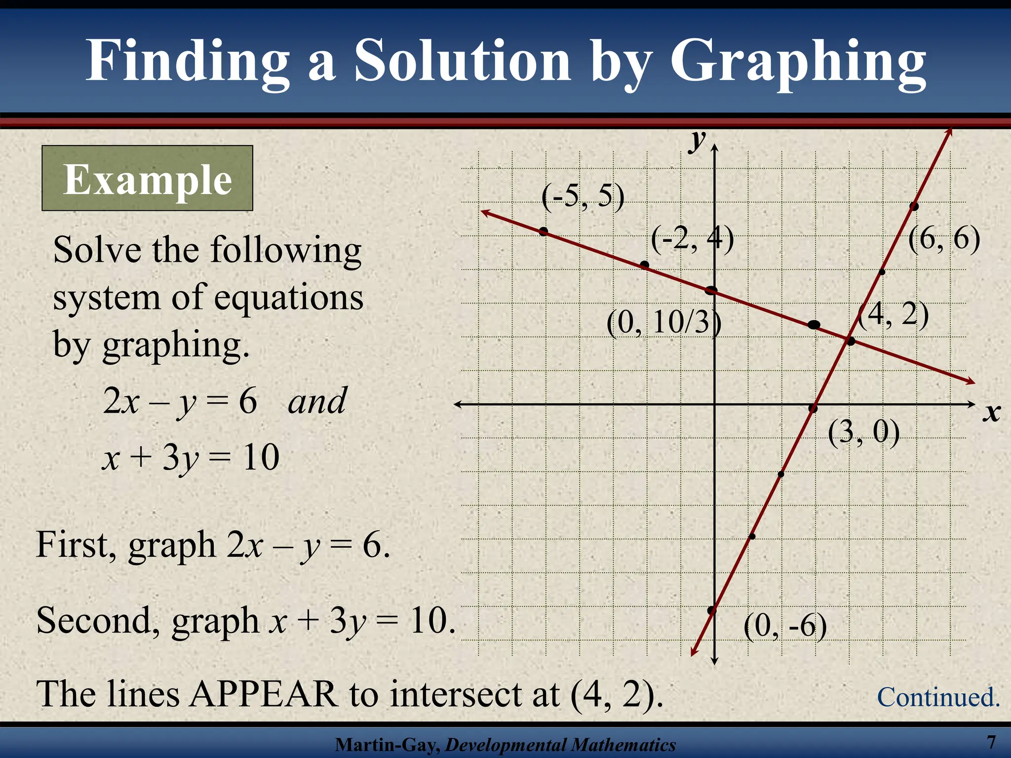
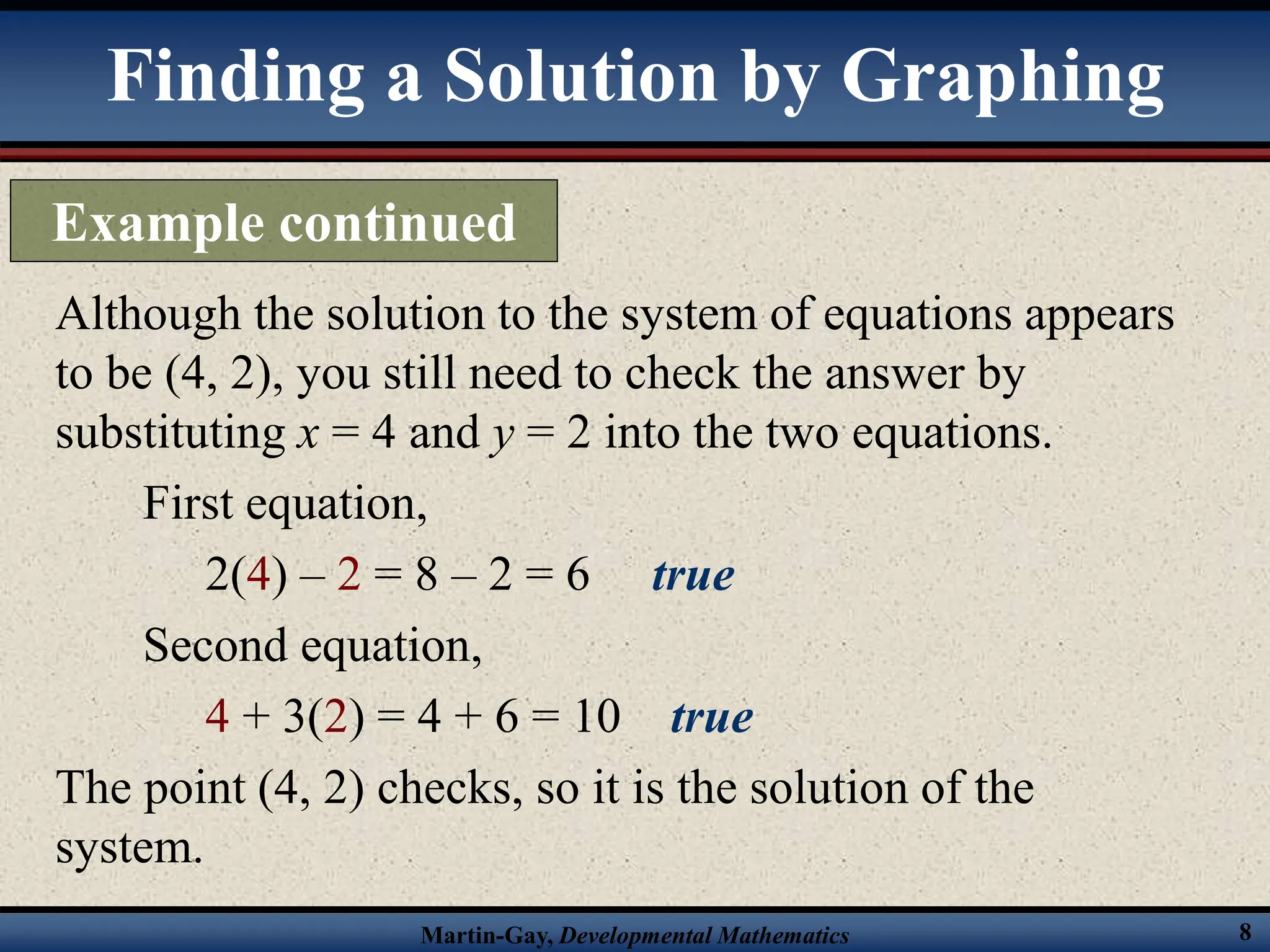
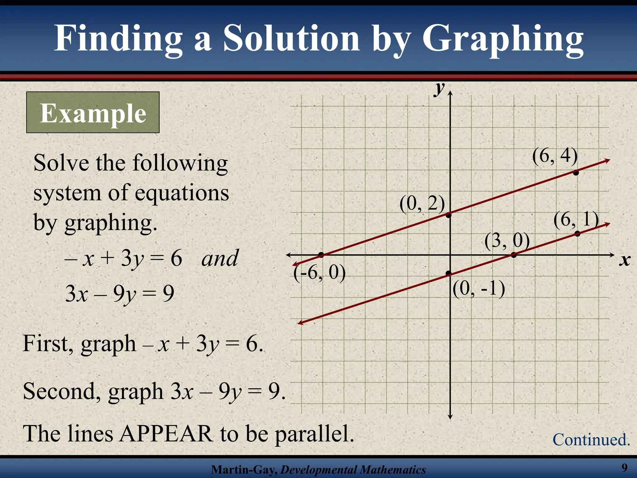
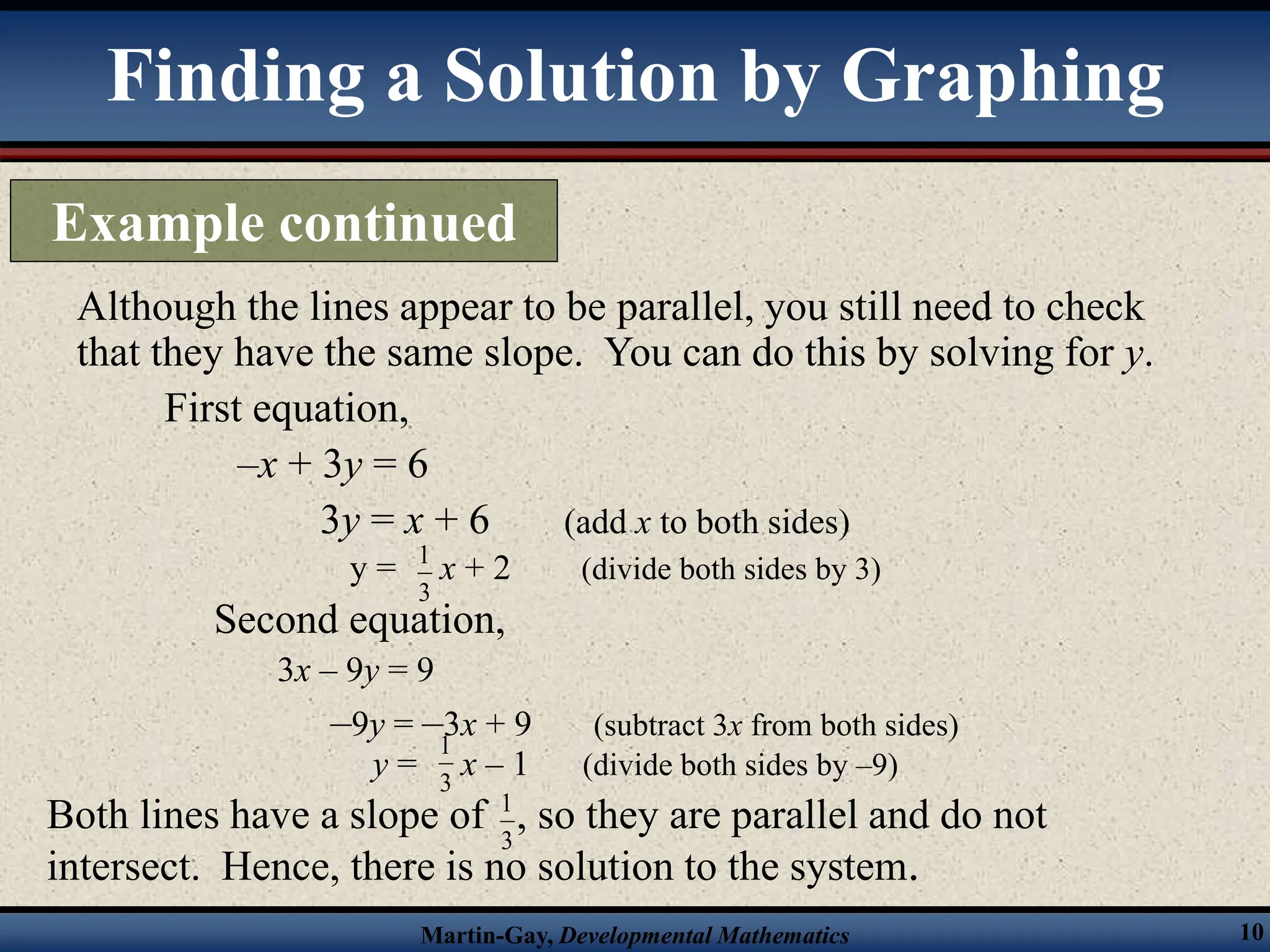
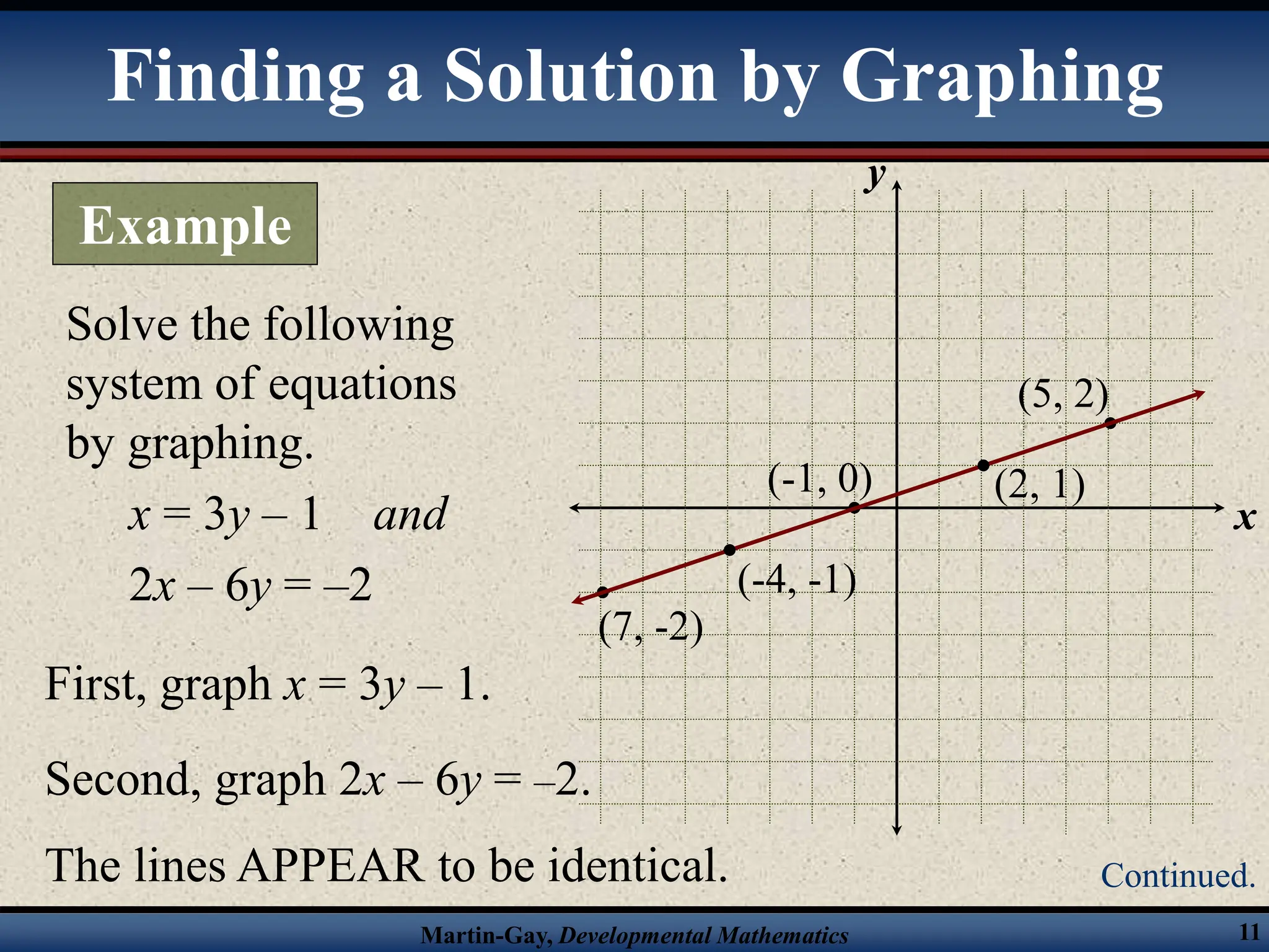
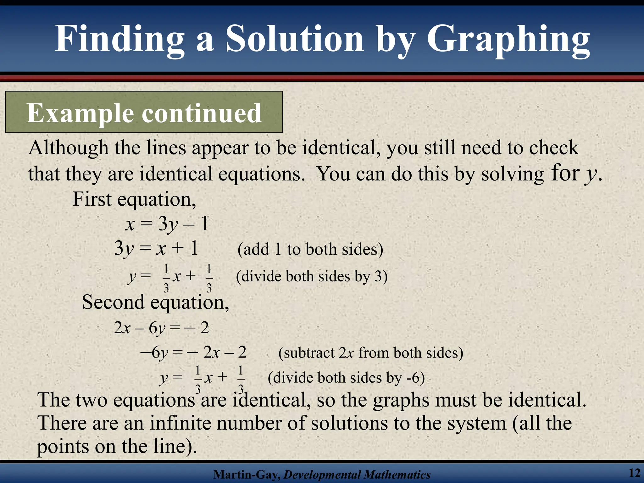
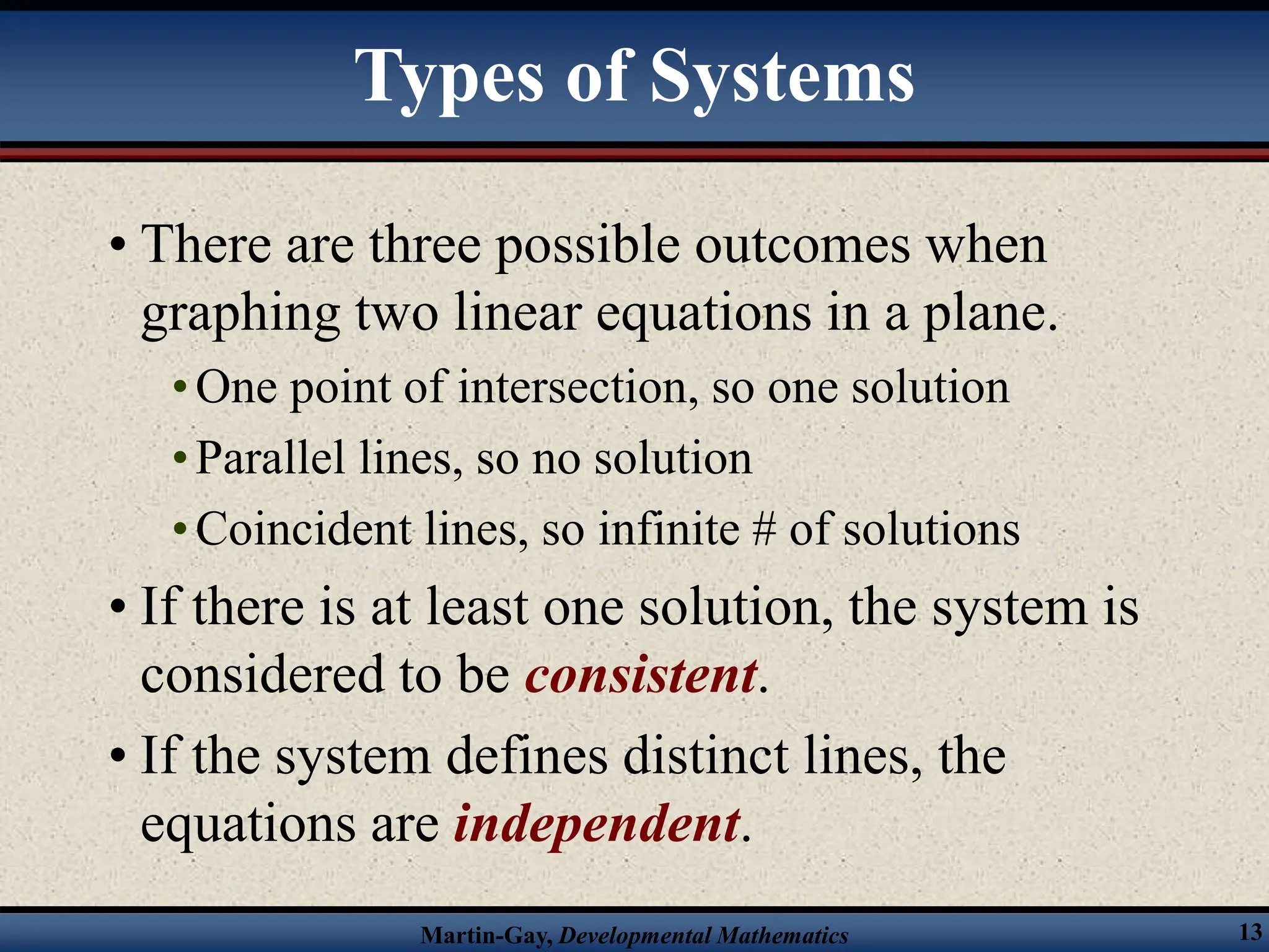
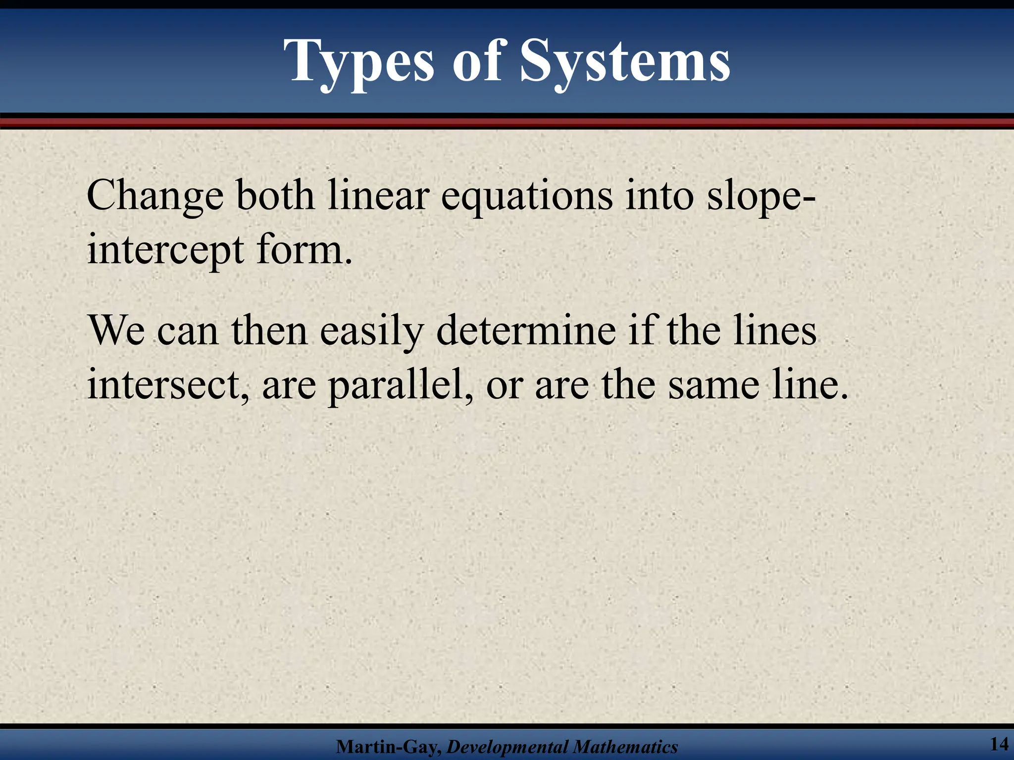
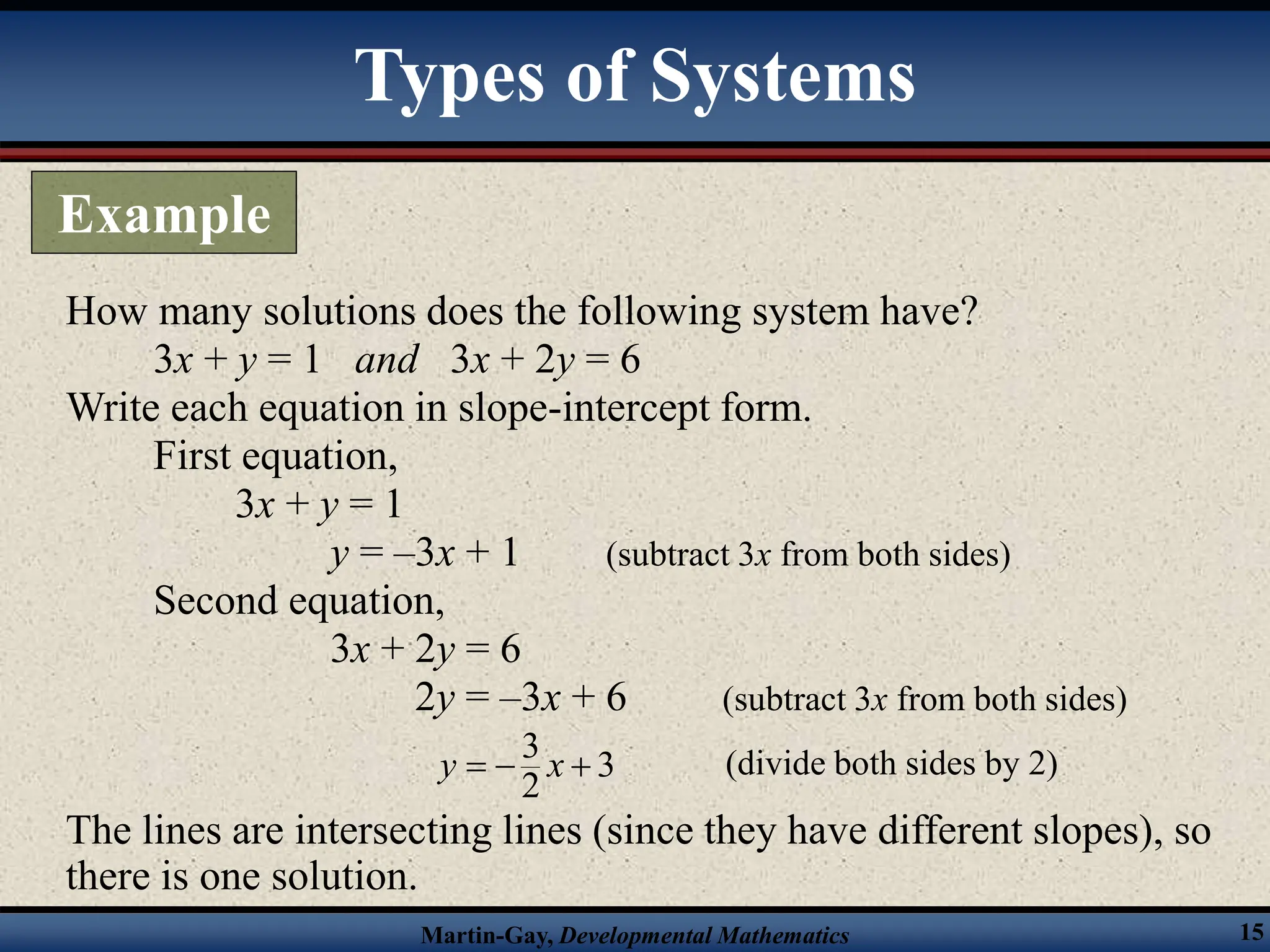
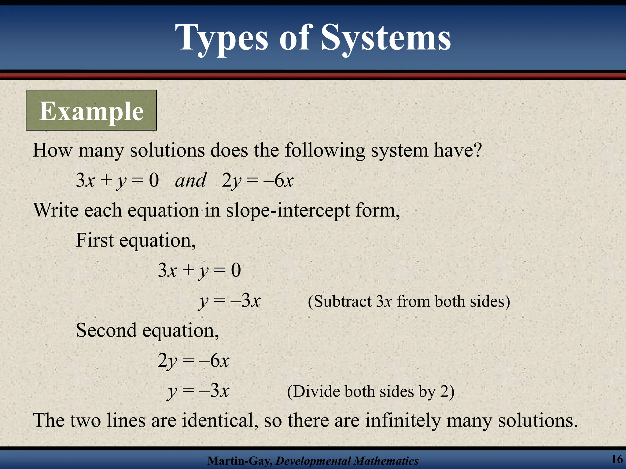
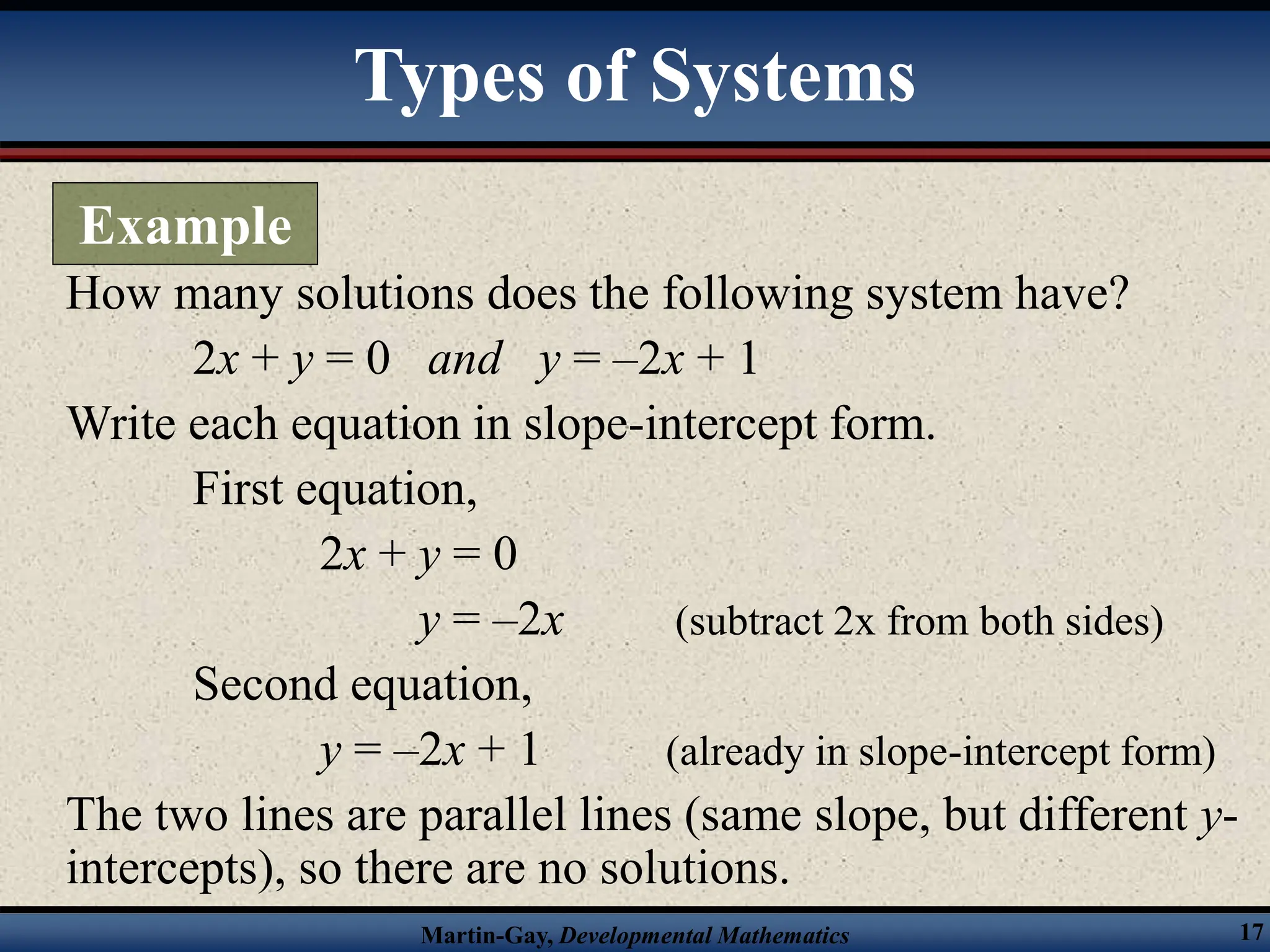
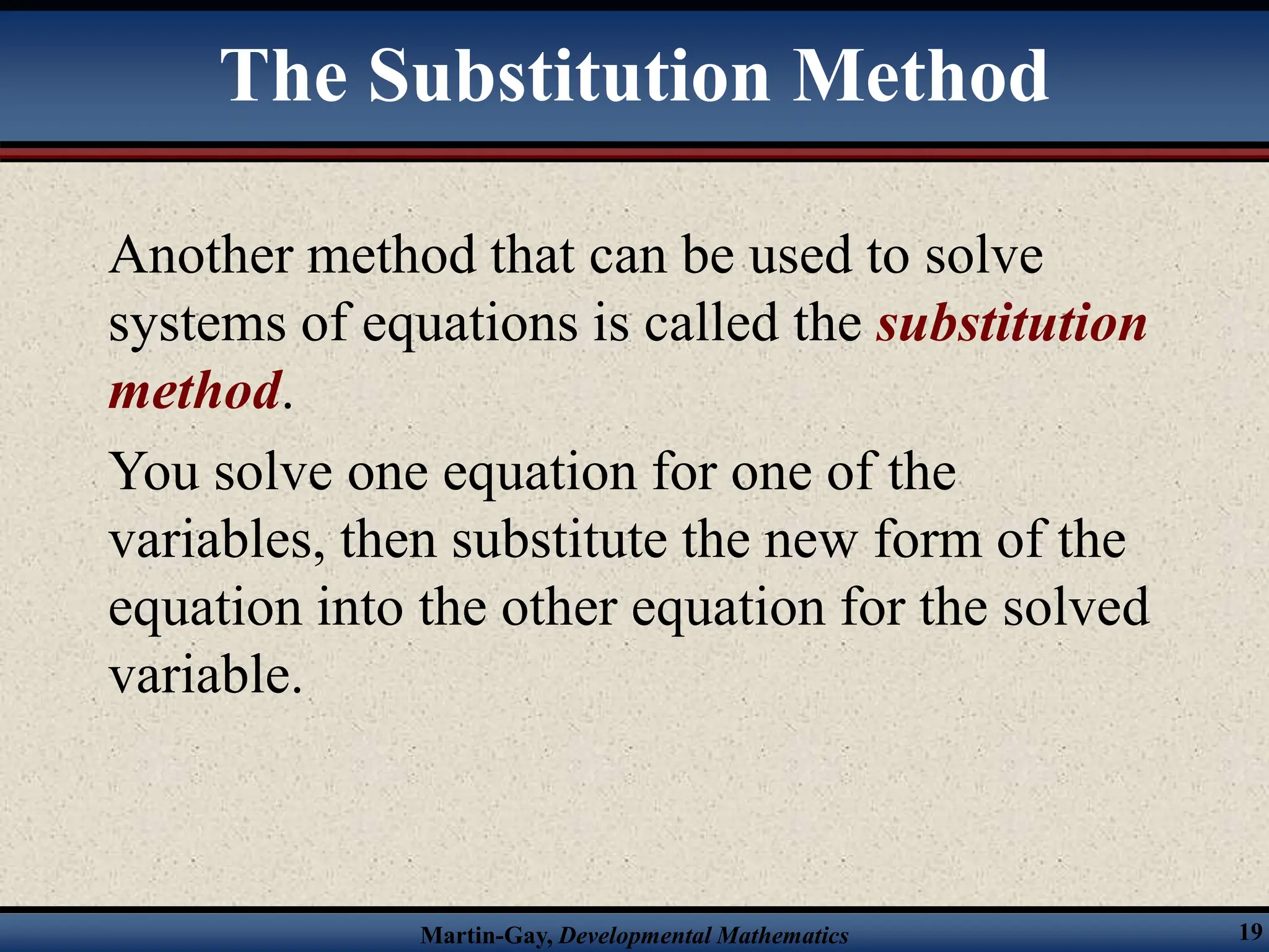
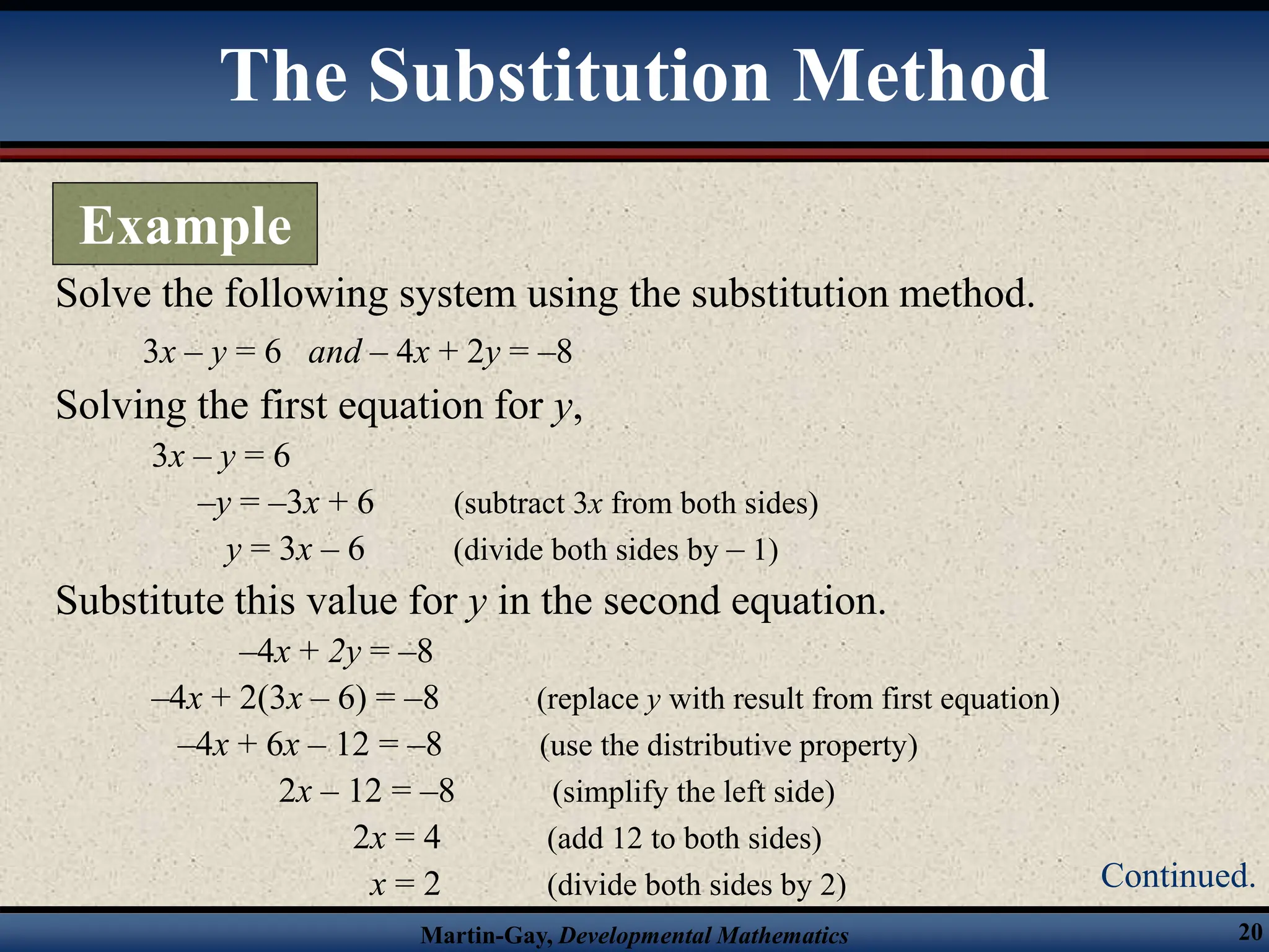
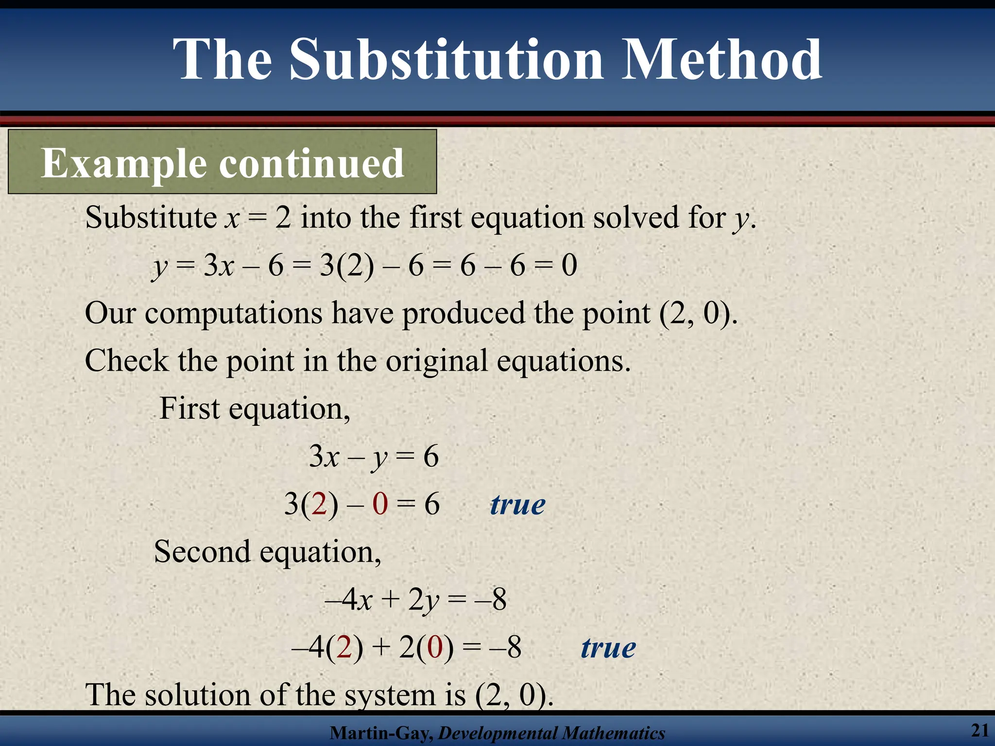
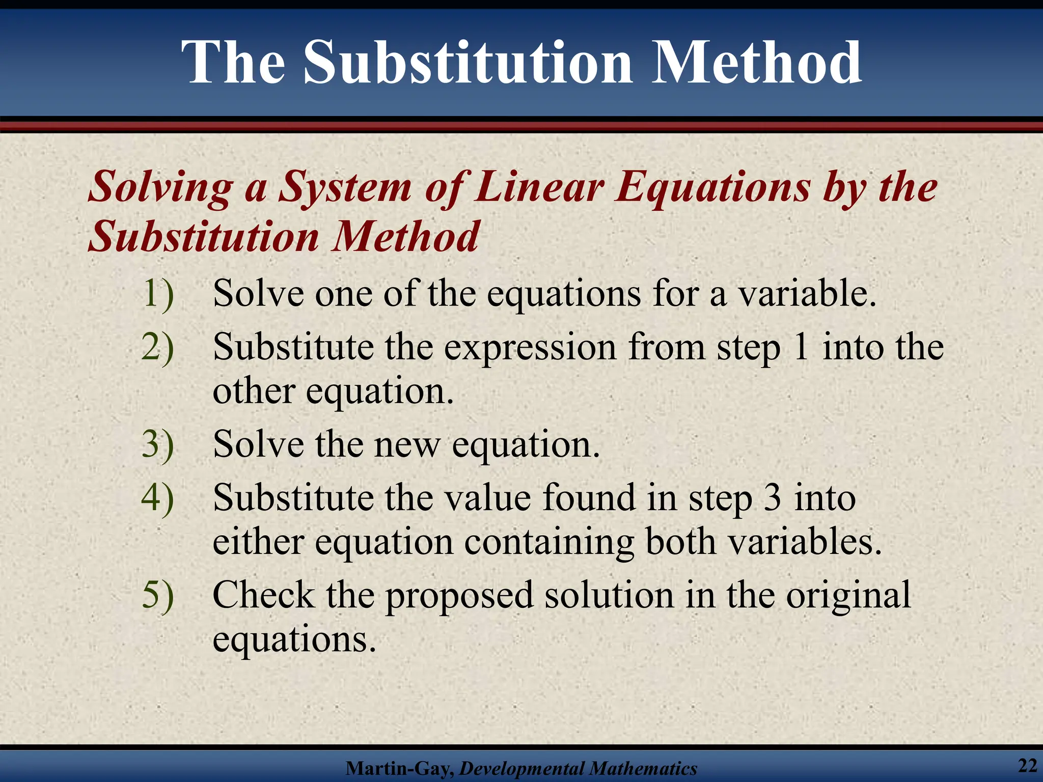
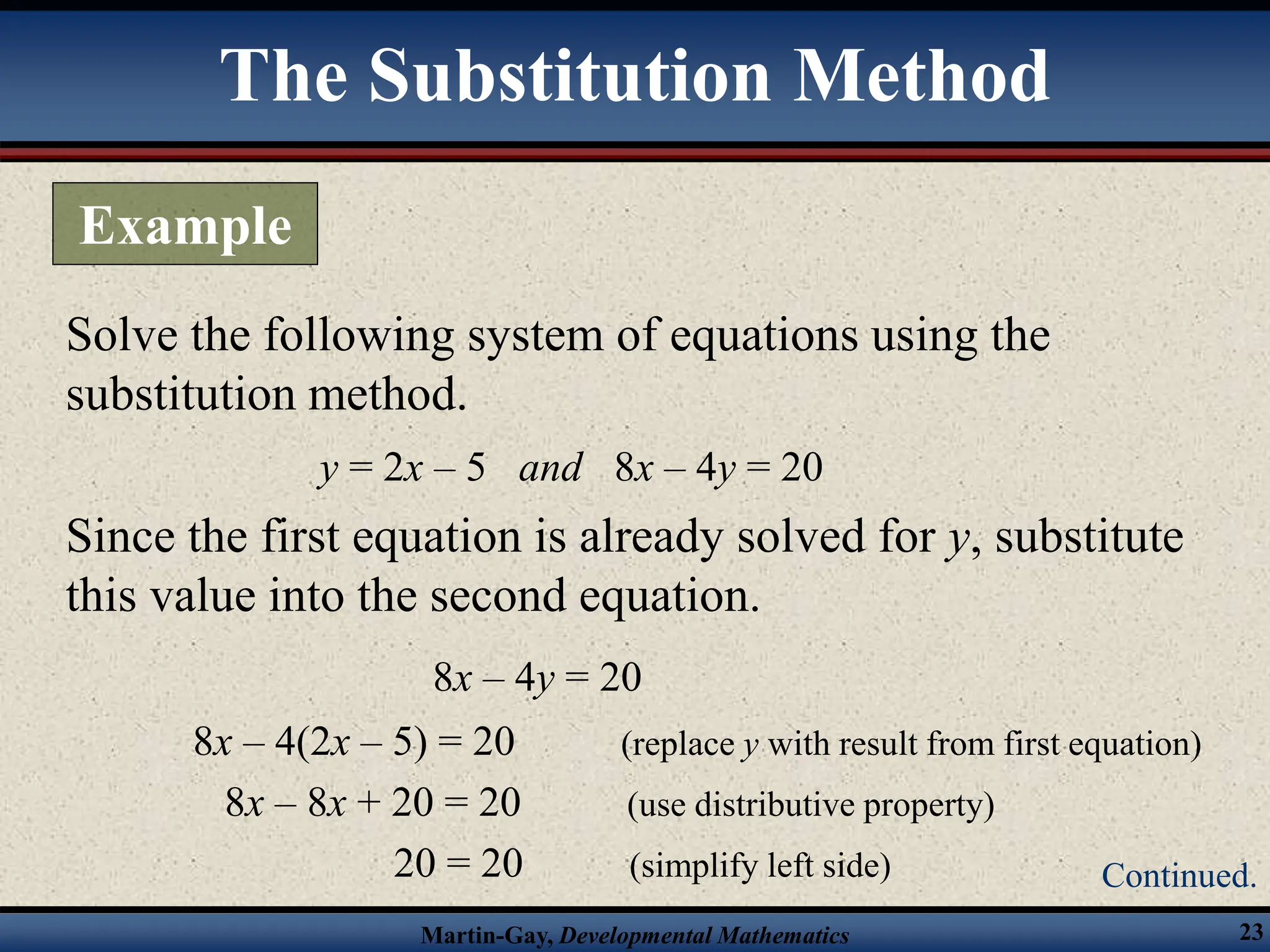
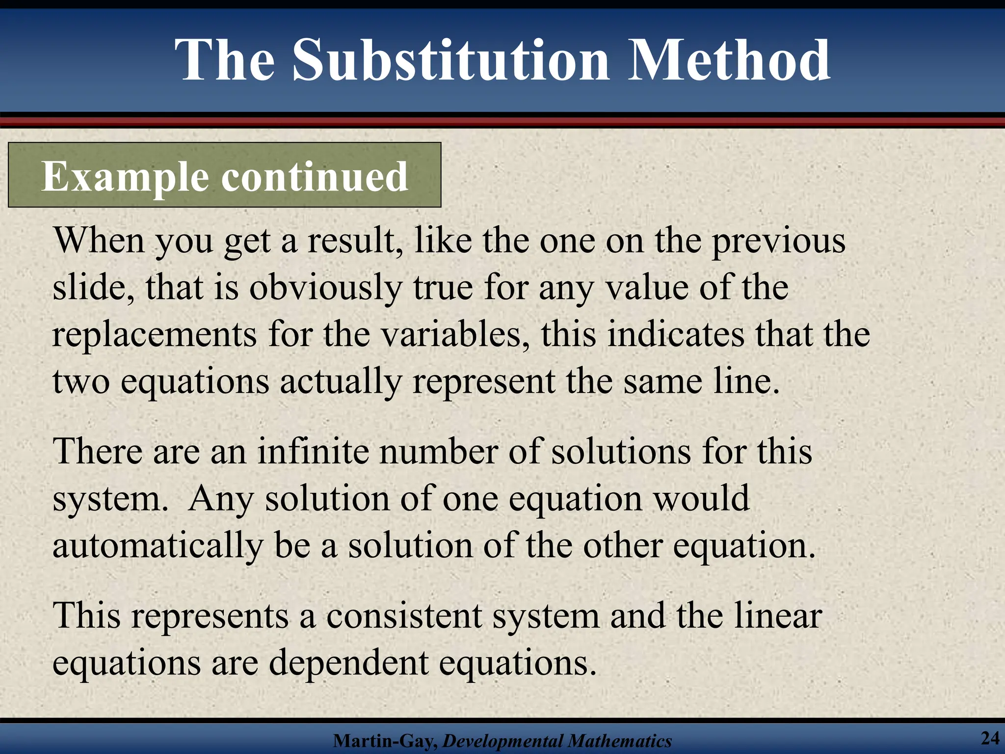
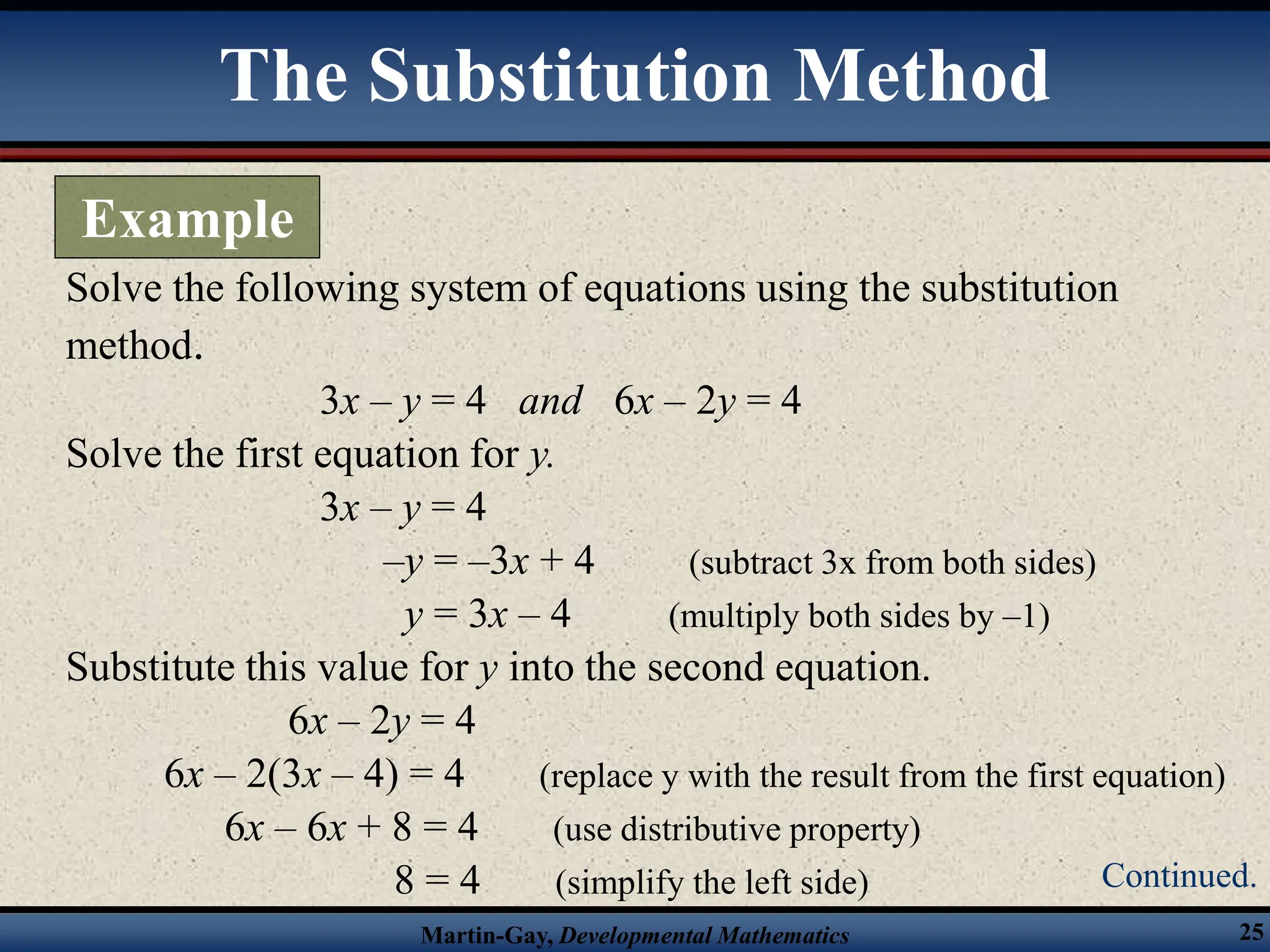
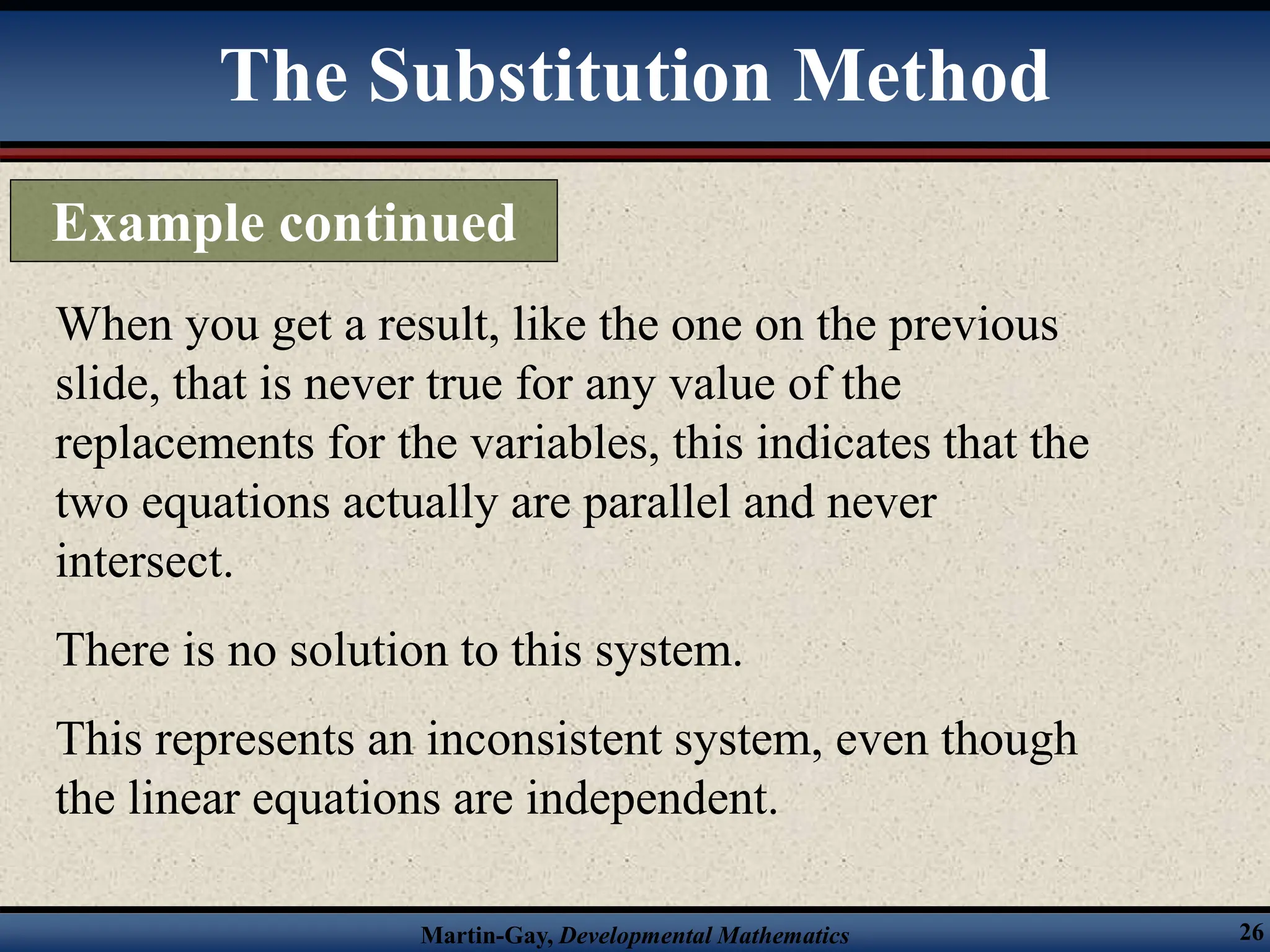
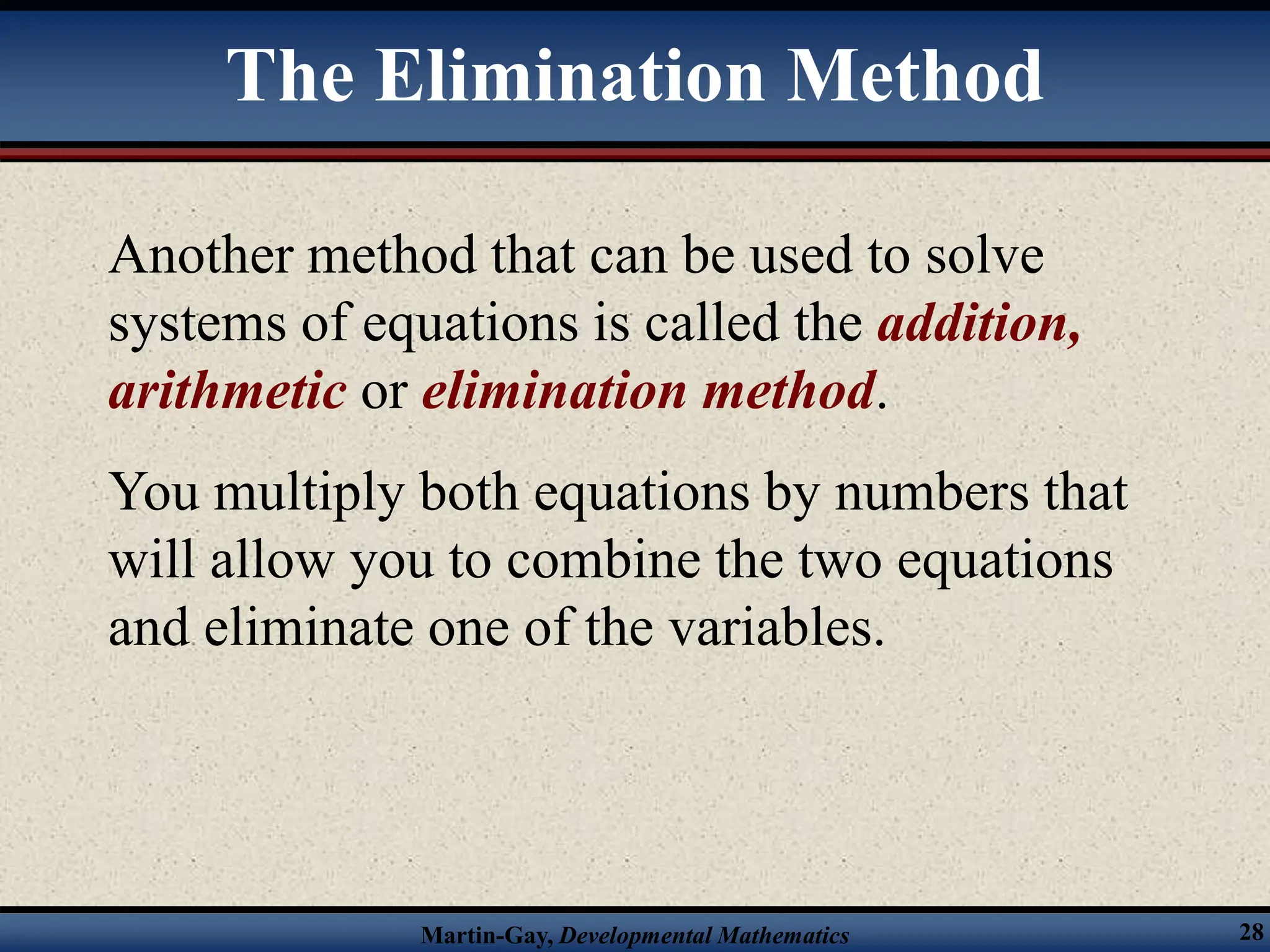
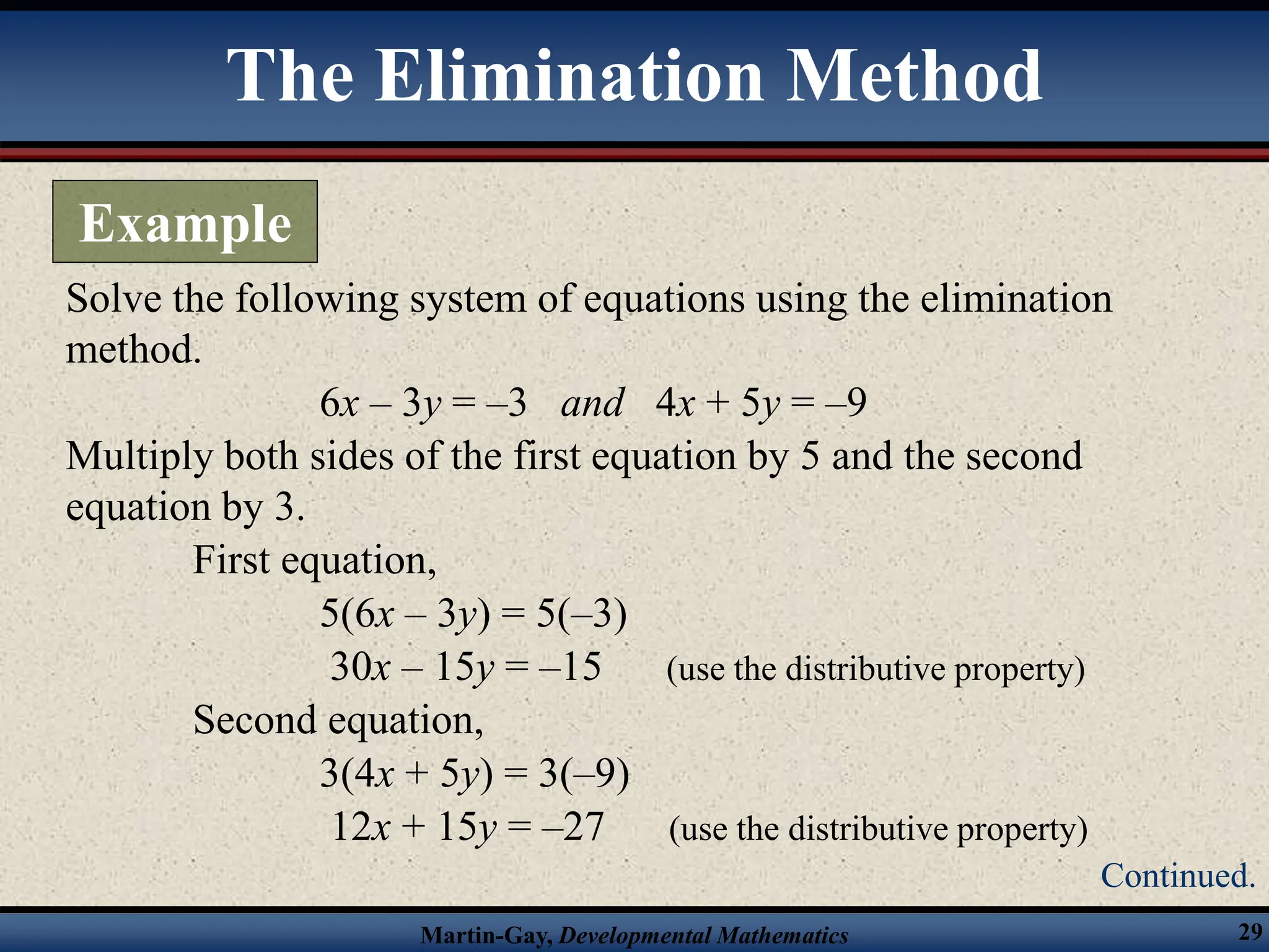
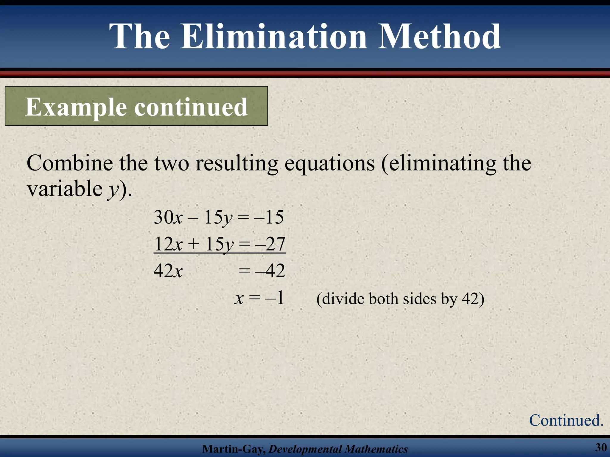
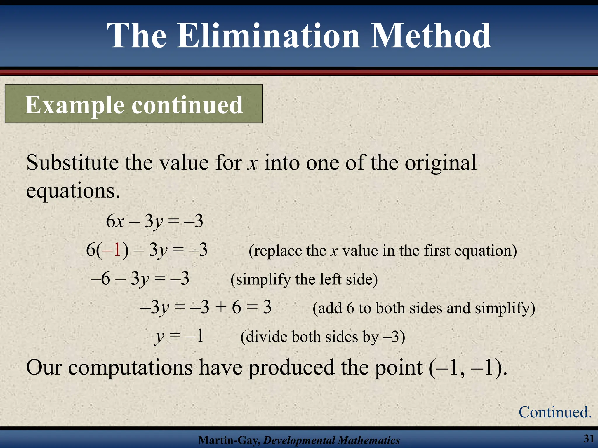
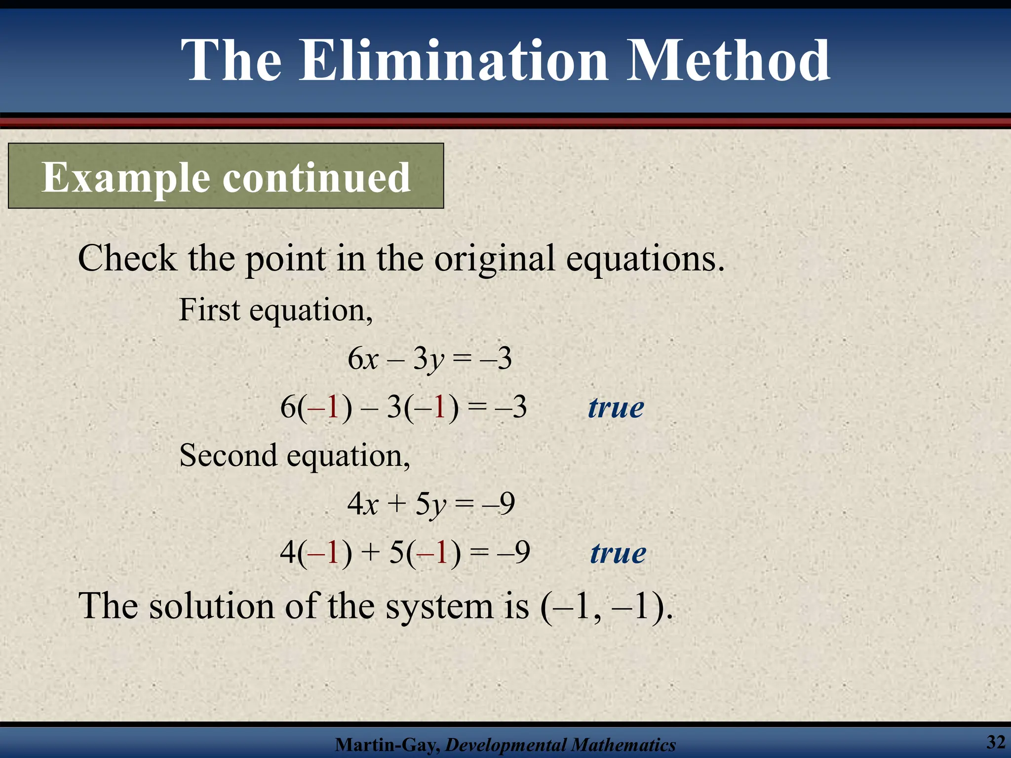
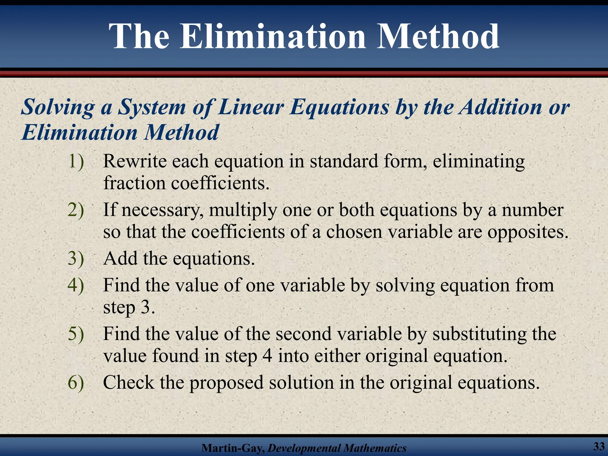
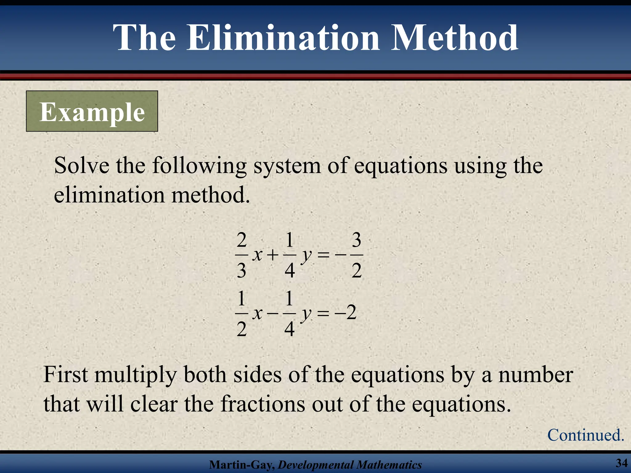
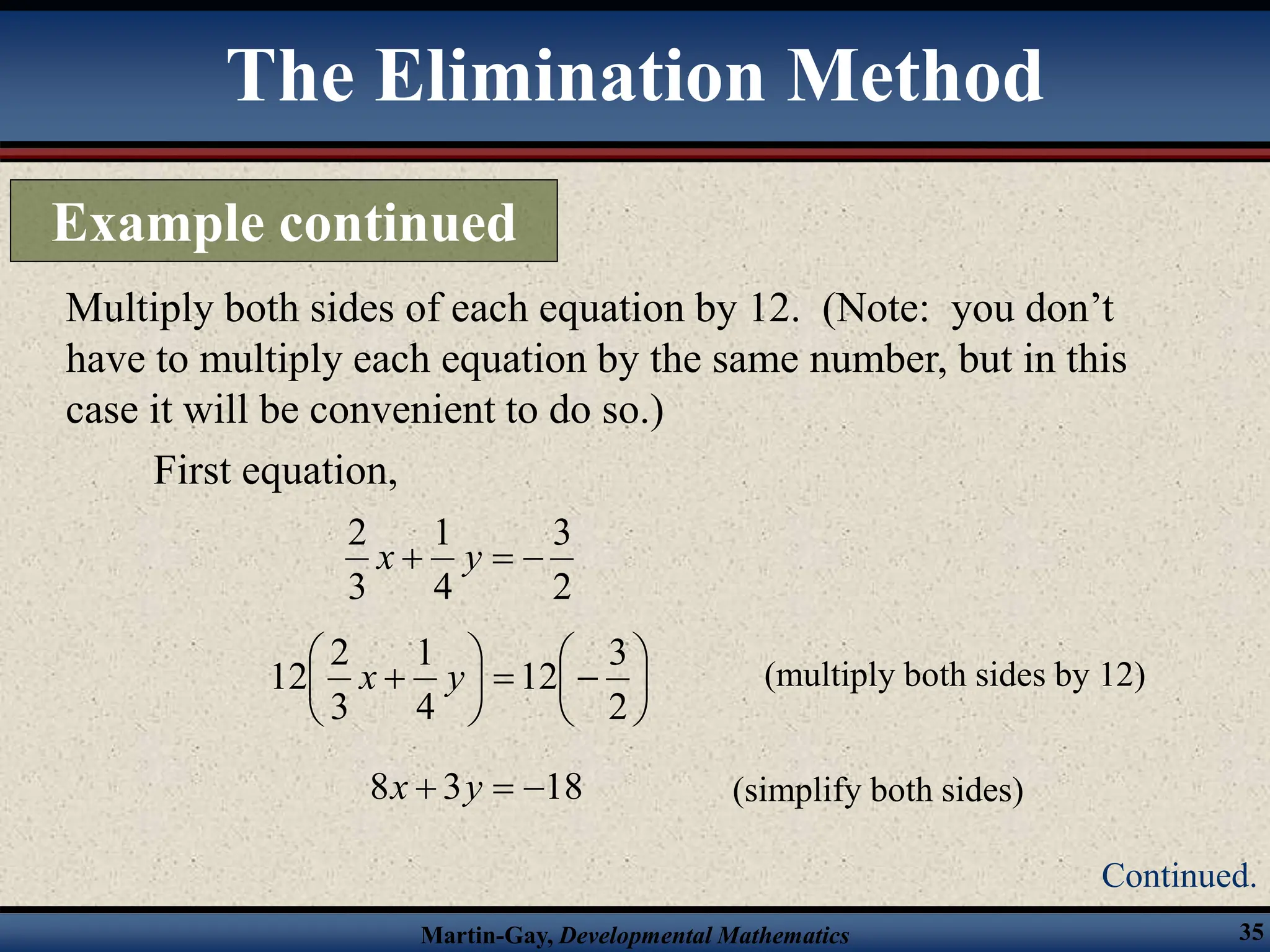
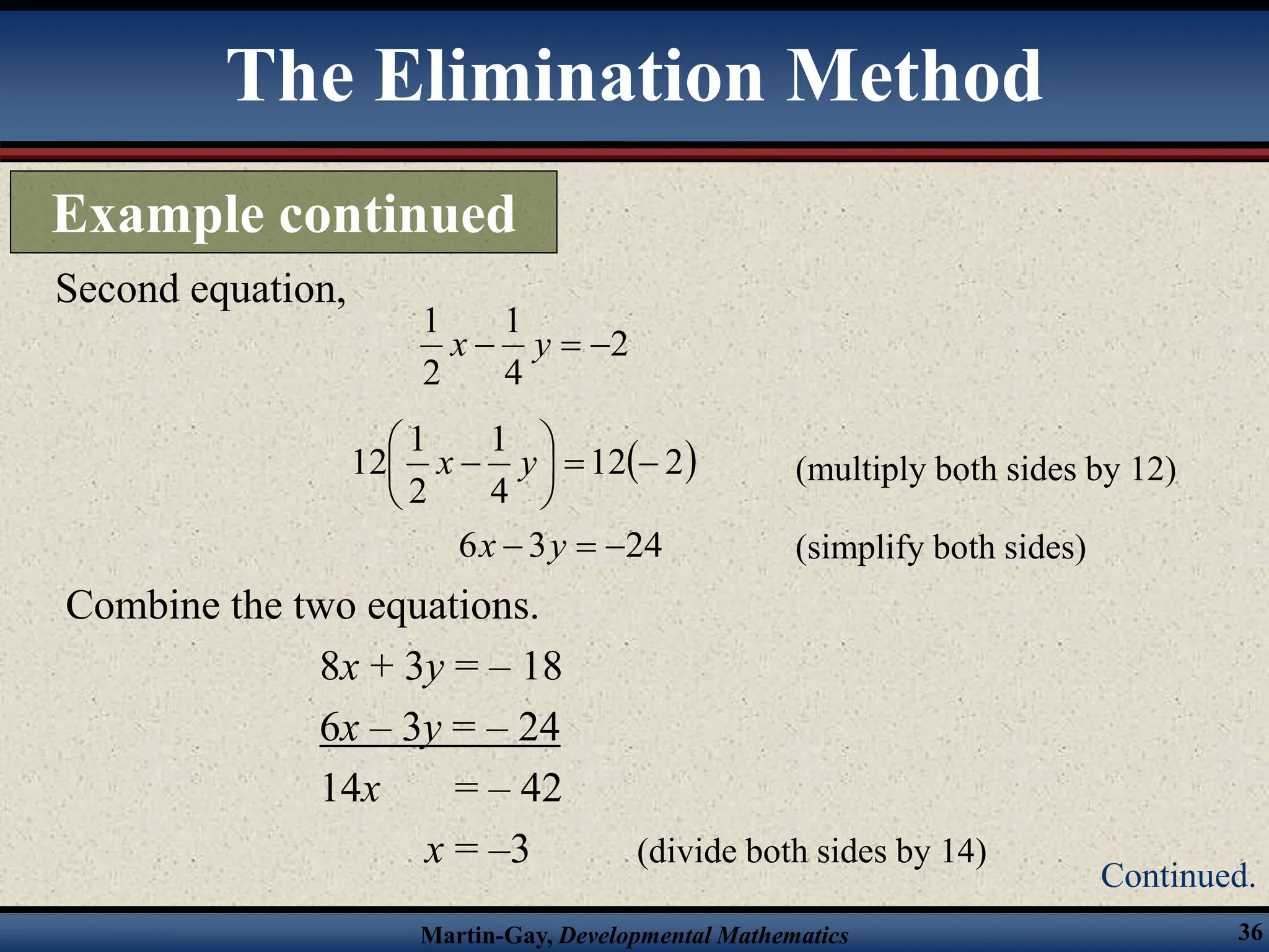
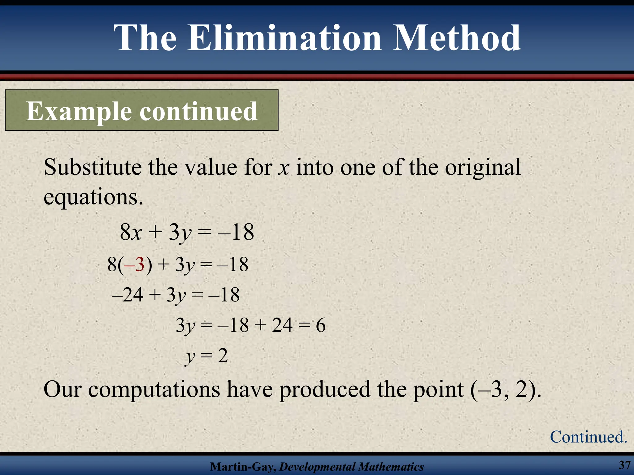
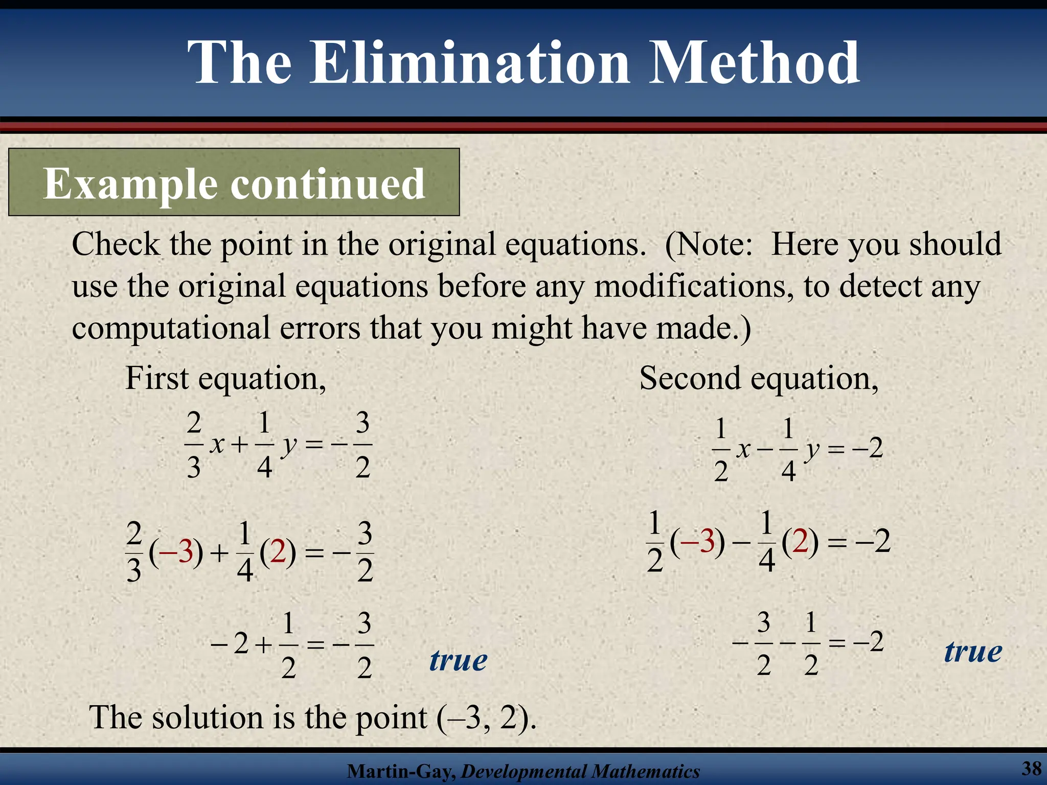
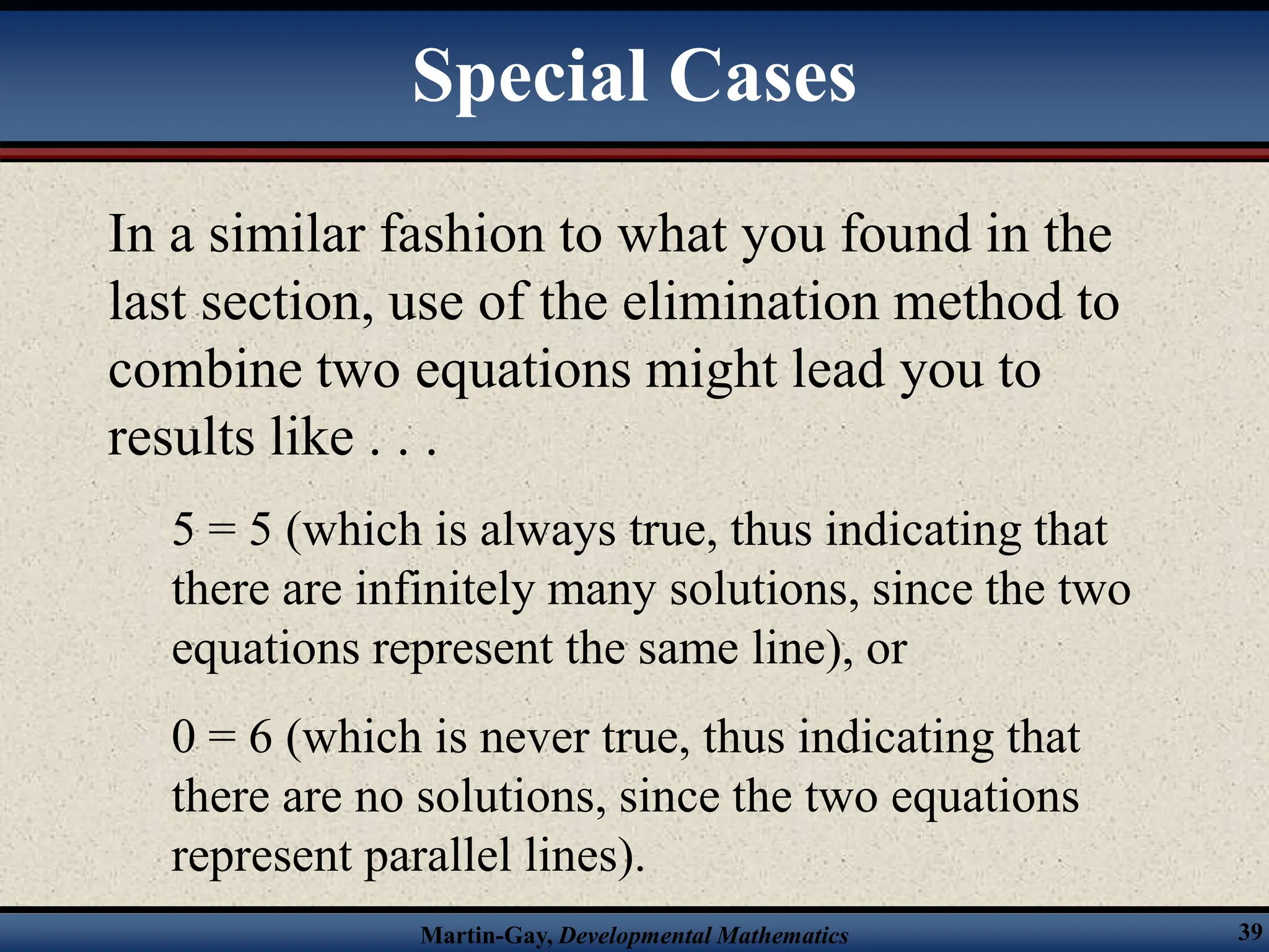
Chapter 3
Systems of
Equations

Solving Systems of Linear
Equations by Graphing

Martin-Gay, Developmental Mathematics 3
Systems of Linear Equations
A system of linear equations consists of two
or more linear equations.
This section focuses on only two equations at
a time.
The solution of a system of linear equations in
two variables is any ordered pair that solves
both of the linear equations.

Determine whether the given point is a solution of the following
system.
point: (– 3, 1)
system: x – y = – 4 and 2x + 10y = 4
•Plug the values into the equations.
First equation: – 3 – 1 = – 4 true
Second equation: 2(– 3) + 10(1) = – 6 + 10 = 4 true
•Since the point (– 3, 1) produces a true statement in both
equations, it is a solution.
Solution of a System
Example

Determine whether the given point is a solution of the following
system
point: (4, 2)
system: 2x – 5y = – 2 and 3x + 4y = 4
Plug the values into the equations
First equation: 2(4) – 5(2) = 8 – 10 = – 2 true
Second equation: 3(4) + 4(2) = 12 + 8 = 20  4 false
Since the point (4, 2) produces a true statement in only one
equation, it is NOT a solution.
Solution of a System
Example

• Since our chances of guessing the right coordinates
to try for a solution are not that high, we’ll be more
successful if we try a different technique.
• Since a solution of a system of equations is a
solution common to both equations, it would also
be a point common to the graphs of both equations.
• So to find the solution of a system of 2 linear
equations, graph the equations and see where the
lines intersect.
Finding a Solution by Graphing

Solve the following
system of equations
by graphing.
2x – y = 6 and
x + 3y = 10
x
y
First, graph 2x – y = 6.
(0, -6)
(3, 0)
(6, 6)
Second, graph x + 3y = 10.
(0, 10/3)
(-2, 4)
(-5, 5)
The lines APPEAR to intersect at (4, 2).
(4, 2)
Example
Continued.

Although the solution to the system of equations appears
to be (4, 2), you still need to check the answer by
substituting x = 4 and y = 2 into the two equations.
First equation,
2(4) – 2 = 8 – 2 = 6 true
Second equation,
4 + 3(2) = 4 + 6 = 10 true
The point (4, 2) checks, so it is the solution of the
system.
Example continued

Solve the following
system of equations
by graphing.
– x + 3y = 6 and
3x – 9y = 9
x
y
First, graph – x + 3y = 6.
(-6, 0)
(0, 2)
(6, 4)
Second, graph 3x – 9y = 9.
(0, -1)
(6, 1)
(3, 0)
The lines APPEAR to be parallel.
Example
Continued.

Although the lines appear to be parallel, you still need to check
that they have the same slope. You can do this by solving for y.
First equation,
–x + 3y = 6
3y = x + 6 (add x to both sides)
3
1
y = x + 2 (divide both sides by 3)
Second equation,
3x – 9y = 9
–9y = –3x + 9 (subtract 3x from both sides)
3
1
y = x – 1 (divide both sides by –9)
3
1
Both lines have a slope of , so they are parallel and do not
intersect. Hence, there is no solution to the system.
Example continued

Solve the following
system of equations
by graphing.
x = 3y – 1 and
2x – 6y = –2
x
y
First, graph x = 3y – 1.
(-1, 0)
(5, 2)
(7, -2)
Second, graph 2x – 6y = –2.
(-4, -1)
(2, 1)
The lines APPEAR to be identical.
Example
Continued.

Although the lines appear to be identical, you still need to check
that they are identical equations. You can do this by solving for y.
First equation,
x = 3y – 1
3y = x + 1 (add 1 to both sides)
Second equation,
2x – 6y = – 2
–6y = – 2x – 2 (subtract 2x from both sides)
The two equations are identical, so the graphs must be identical.
There are an infinite number of solutions to the system (all the
points on the line).
3
1
y = x + (divide both sides by 3)
3
1
3
1
y = x + (divide both sides by -6)
3
1
Example continued

• There are three possible outcomes when
graphing two linear equations in a plane.
•One point of intersection, so one solution
•Parallel lines, so no solution
•Coincident lines, so infinite # of solutions
• If there is at least one solution, the system is
considered to be consistent.
• If the system defines distinct lines, the
equations are independent.
Types of Systems

Change both linear equations into slope-
intercept form.
We can then easily determine if the lines
intersect, are parallel, or are the same line.
Types of Systems

How many solutions does the following system have?
3x + y = 1 and 3x + 2y = 6
Write each equation in slope-intercept form.
First equation,
3x + y = 1
y = –3x + 1 (subtract 3x from both sides)
Second equation,
3x + 2y = 6
2y = –3x + 6 (subtract 3x from both sides)
The lines are intersecting lines (since they have different slopes), so
there is one solution.
(divide both sides by 2)
3
3
2
y x
  
Types of Systems
Example

3x + y = 0 and 2y = –6x
Write each equation in slope-intercept form,
First equation,
3x + y = 0
y = –3x (Subtract 3x from both sides)
Second equation,
2y = –6x
y = –3x (Divide both sides by 2)
The two lines are identical, so there are infinitely many solutions.
Types of Systems
Example

2x + y = 0 and y = –2x + 1
Write each equation in slope-intercept form.
First equation,
2x + y = 0
y = –2x (subtract 2x from both sides)
Second equation,
y = –2x + 1 (already in slope-intercept form)
The two lines are parallel lines (same slope, but different y-
intercepts), so there are no solutions.
Types of Systems
Example

Equations by Substitution

The Substitution Method
Another method that can be used to solve
systems of equations is called the substitution
method.
You solve one equation for one of the
variables, then substitute the new form of the
equation into the other equation for the solved
variable.

Solve the following system using the substitution method.
3x – y = 6 and – 4x + 2y = –8
Solving the first equation for y,
3x – y = 6
–y = –3x + 6 (subtract 3x from both sides)
y = 3x – 6 (divide both sides by – 1)
Substitute this value for y in the second equation.
–4x + 2y = –8
–4x + 2(3x – 6) = –8 (replace y with result from first equation)
–4x + 6x – 12 = –8 (use the distributive property)
2x – 12 = –8 (simplify the left side)
2x = 4 (add 12 to both sides)
x = 2 (divide both sides by 2)
Example
Continued.

Substitute x = 2 into the first equation solved for y.
y = 3x – 6 = 3(2) – 6 = 6 – 6 = 0
Our computations have produced the point (2, 0).
Check the point in the original equations.
First equation,
3x – y = 6
3(2) – 0 = 6 true
Second equation,
–4x + 2y = –8
–4(2) + 2(0) = –8 true
The solution of the system is (2, 0).
Example continued

Solving a System of Linear Equations by the
Substitution Method
1) Solve one of the equations for a variable.
2) Substitute the expression from step 1 into the
other equation.
3) Solve the new equation.
4) Substitute the value found in step 3 into
either equation containing both variables.
5) Check the proposed solution in the original
equations.

Solve the following system of equations using the
substitution method.
y = 2x – 5 and 8x – 4y = 20
Since the first equation is already solved for y, substitute
this value into the second equation.
8x – 4y = 20
8x – 4(2x – 5) = 20 (replace y with result from first equation)
8x – 8x + 20 = 20 (use distributive property)
20 = 20 (simplify left side)
Example
Continued.

When you get a result, like the one on the previous
slide, that is obviously true for any value of the
replacements for the variables, this indicates that the
two equations actually represent the same line.
There are an infinite number of solutions for this
system. Any solution of one equation would
automatically be a solution of the other equation.
This represents a consistent system and the linear
equations are dependent equations.
Example continued

Solve the following system of equations using the substitution
method.
3x – y = 4 and 6x – 2y = 4
Solve the first equation for y.
3x – y = 4
–y = –3x + 4 (subtract 3x from both sides)
y = 3x – 4 (multiply both sides by –1)
Substitute this value for y into the second equation.
6x – 2y = 4
6x – 2(3x – 4) = 4 (replace y with the result from the first equation)
6x – 6x + 8 = 4 (use distributive property)
8 = 4 (simplify the left side)
Example
Continued.

When you get a result, like the one on the previous
slide, that is never true for any value of the
replacements for the variables, this indicates that the
two equations actually are parallel and never
intersect.
There is no solution to this system.
This represents an inconsistent system, even though
the linear equations are independent.
Example continued

Equations by Elimination

The Elimination Method
Another method that can be used to solve
systems of equations is called the addition,
arithmetic or elimination method.
You multiply both equations by numbers that
will allow you to combine the two equations
and eliminate one of the variables.

Solve the following system of equations using the elimination
method.
6x – 3y = –3 and 4x + 5y = –9
Multiply both sides of the first equation by 5 and the second
equation by 3.
First equation,
5(6x – 3y) = 5(–3)
30x – 15y = –15 (use the distributive property)
Second equation,
3(4x + 5y) = 3(–9)
12x + 15y = –27 (use the distributive property)
Example
Continued.

Combine the two resulting equations (eliminating the
variable y).
30x – 15y = –15
12x + 15y = –27
42x = –42
x = –1 (divide both sides by 42)
Example continued
Continued.

Substitute the value for x into one of the original
equations.
6x – 3y = –3
6(–1) – 3y = –3 (replace the x value in the first equation)
–6 – 3y = –3 (simplify the left side)
–3y = –3 + 6 = 3 (add 6 to both sides and simplify)
y = –1 (divide both sides by –3)
Our computations have produced the point (–1, –1).
Example continued
Continued.

Check the point in the original equations.
First equation,
6x – 3y = –3
6(–1) – 3(–1) = –3 true
Second equation,
4x + 5y = –9
4(–1) + 5(–1) = –9 true
The solution of the system is (–1, –1).
Example continued

Solving a System of Linear Equations by the Addition or
Elimination Method
1) Rewrite each equation in standard form, eliminating
fraction coefficients.
2) If necessary, multiply one or both equations by a number
so that the coefficients of a chosen variable are opposites.
3) Add the equations.
4) Find the value of one variable by solving equation from
step 3.
5) Find the value of the second variable by substituting the
value found in step 4 into either original equation.
6) Check the proposed solution in the original equations.

Solve the following system of equations using the
elimination method.
2
4
1
2
1
2
3
4
1
3
2






y
x
y
x
First multiply both sides of the equations by a number
that will clear the fractions out of the equations.
Example
Continued.

Multiply both sides of each equation by 12. (Note: you don’t
have to multiply each equation by the same number, but in this
case it will be convenient to do so.)
First equation,
2
3
4
1
3
2


 y
x















2
3
12
4
1
3
2
12 y
x (multiply both sides by 12)
18
3
8 

 y
x (simplify both sides)
Example continued
Continued.

Combine the two equations.
8x + 3y = – 18
6x – 3y = – 24
14x = – 42
x = –3 (divide both sides by 14)
Second equation,
2
4
1
2
1


 y
x
 
2
12
4
1
2
1
12 







 y
x (multiply both sides by 12)
(simplify both sides)
24
3
6 

 y
x
Example continued
Continued.

Substitute the value for x into one of the original
equations.
8x + 3y = –18
8(–3) + 3y = –18
–24 + 3y = –18
3y = –18 + 24 = 6
y = 2
Our computations have produced the point (–3, 2).
Example continued
Continued.

Check the point in the original equations. (Note: Here you should
use the original equations before any modifications, to detect any
computational errors that you might have made.)
First equation,
2
3
4
1
3
2


 y
x
2 1 3
( ) ( )
3 4 2
3 2
  

2
3
2
1
2 



true
Second equation,
2
4
1
2
1


 y
x
1 1
( ) ( ) 2
2 4
3 2
  

2
2
1
2
3



 true
The solution is the point (–3, 2).
Example continued

In a similar fashion to what you found in the
last section, use of the elimination method to
combine two equations might lead you to
results like . . .
5 = 5 (which is always true, thus indicating that
there are infinitely many solutions, since the two
equations represent the same line), or
0 = 6 (which is never true, thus indicating that
there are no solutions, since the two equations
represent parallel lines).
Special Cases

systems of equations.ppt

More Related Content

What's hot

Similar to systems of equations.ppt

More from JennilynBalusdan3

Recently uploaded

In this document

systems of equations.ppt