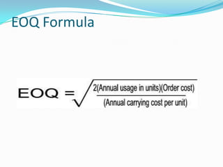
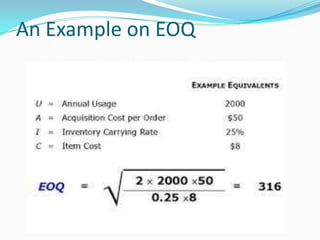
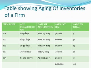
What is EOQ?
 Quantity of materials which can be purchased at

minimum costs.
 It is the size of the lot to be purchased which is

economically viable.
 The framework used to determine this order quantity is

also known as Wilson EOQ Model or Wilson Formula.
 In determining EOQ, it is assumed that cost of

managing inventory is made up solely of two parts i.e.,
a) Ordering costs/ Buying costs
b) Carrying costs/ Holding costs
Ordering Costs/ Buying Costs
 Costs which are associated with the purchasing or ordering of

materials.
 These costs include:

a) Costs of staff posted for ordering of goods.
b) Expenses incurred on transportation of goods purchased.

c) Inspection costs of incoming materials.
d) Cost of stationary, typing, postage, telephone charges, etc.
Carrying Costs
 Costs for holding the inventories.
 These costs include :

a) the cost of capital invested in inventories.
b) cost of storage which could have been used for other
purposes.

c) the loss of materials due to deterioration and obsolescence.
d) insurance costs.
e) cost of spoilage in handling of materials.
Assumptions of EOQ Model
 The ordering cost is constant.
 The rate of demand is known, and spread evenly throughout

the year.
 The lead time is fixed.
 The purchase price of the item is constant i.e. no discount is

available.
 The replenishment is made instantaneously, the whole batch is

delivered at once.
EOQ Formula
An Example on EOQ
What is Aging Schedule of
Inventories?
 Classification of inventories according to the period (age)

of their holding.
 Helps in identifying slow moving inventories thereby

helping in effective control and management of
inventories
Table showing Aging Of Inventories
of a Firm
ITEM CODE

AGE
CLASSIFICATI
ON

DATE OF
AMOUNT
ACQUISITION (RS.)

%AGE TO
TOTAL

001

0-15 days

June 25, 2013

30,000

15

002

16-30 days

June 10, 2013

60,000

30

003

31-45 days

May 20, 2013

50,000

25

004

46-60 days

May 5, 2013

40,000

20

005

61 and above

April 12, 2013

20,000

10

2,00,000

100

Economic order quantity (eoq)

  • 2.
    What is EOQ? Quantity of materials which can be purchased at minimum costs.  It is the size of the lot to be purchased which is economically viable.  The framework used to determine this order quantity is also known as Wilson EOQ Model or Wilson Formula.
  • 3.
     In determiningEOQ, it is assumed that cost of managing inventory is made up solely of two parts i.e., a) Ordering costs/ Buying costs b) Carrying costs/ Holding costs
  • 4.
    Ordering Costs/ BuyingCosts  Costs which are associated with the purchasing or ordering of materials.  These costs include: a) Costs of staff posted for ordering of goods. b) Expenses incurred on transportation of goods purchased. c) Inspection costs of incoming materials. d) Cost of stationary, typing, postage, telephone charges, etc.
  • 5.
    Carrying Costs  Costsfor holding the inventories.  These costs include : a) the cost of capital invested in inventories. b) cost of storage which could have been used for other purposes. c) the loss of materials due to deterioration and obsolescence. d) insurance costs. e) cost of spoilage in handling of materials.
  • 6.
    Assumptions of EOQModel  The ordering cost is constant.  The rate of demand is known, and spread evenly throughout the year.  The lead time is fixed.  The purchase price of the item is constant i.e. no discount is available.  The replenishment is made instantaneously, the whole batch is delivered at once.
  • 7.
  • 8.
  • 10.
    What is AgingSchedule of Inventories?  Classification of inventories according to the period (age) of their holding.  Helps in identifying slow moving inventories thereby helping in effective control and management of inventories
  • 11.
    Table showing AgingOf Inventories of a Firm ITEM CODE AGE CLASSIFICATI ON DATE OF AMOUNT ACQUISITION (RS.) %AGE TO TOTAL 001 0-15 days June 25, 2013 30,000 15 002 16-30 days June 10, 2013 60,000 30 003 31-45 days May 20, 2013 50,000 25 004 46-60 days May 5, 2013 40,000 20 005 61 and above April 12, 2013 20,000 10 2,00,000 100