Downloaded 333 times
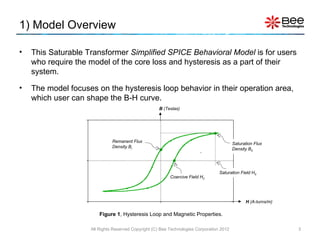
![2) Concept of the Model The Saturable core is characterized by parameters: BSAT, RLOSS, LM and BEXP, which represent the Flux density vs. Magnetic field characteristics of the Saturable core. The Ideal transformer is characterized by parameters: N, R P , R S and L P . Saturable Core Simplified SPICE Behavioral Model [Model parameters: BSAT, RLOSS, LM and BEXP] Ideal Transformer Simplified SPICE Behavioral Model [Model parameters: N, R P , R S and L P ] All Rights Reserved Copyright (C) Bee Technologies Corporation 2012](https://image.slidesharecdn.com/saturabletransformersimplifiedopen-120104070814-phpapp01/85/Simple-Model-of-Transformer-using-LTspice-4-320.jpg)
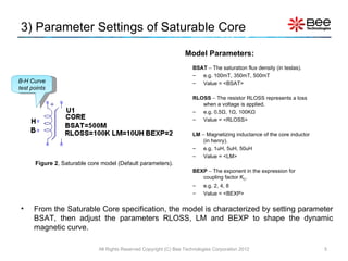
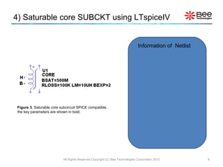
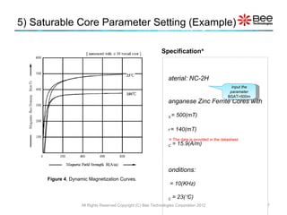
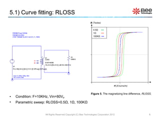
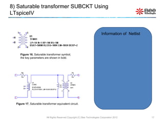
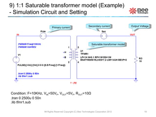
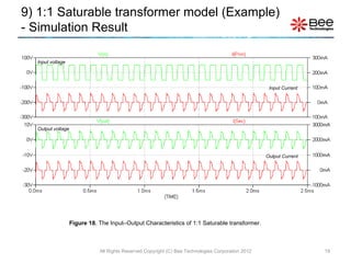
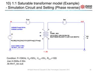

This document describes a simplified SPICE behavioral model for a saturable transformer. It provides an overview of the model concepts and parameters that characterize the saturable core and ideal transformer components of the model. These include BSAT, RLOSS, LM, and BEXP for the core, and N, RP, RS, and LP for the transformer. The document also provides examples of simulations using the model to demonstrate its hysteresis behavior under different excitation conditions.