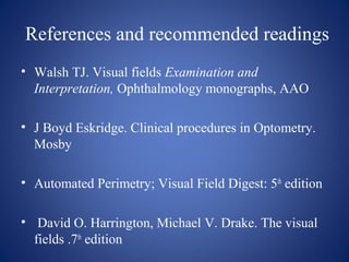
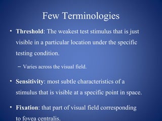

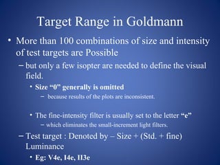
![Goldmann Perimetry: Roman numeral
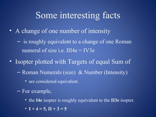
• Sizes of Stimuli [0...V scale]
• Each size increment equals
• a twofold increase in diameter and a fourfold
increase in area.
Diameter (mm) Area (mm2
)
0 0.28 1/16
I 0.56 ¼
II 1.13 1
III 2.26 4
IV 4.51 16
V 9.03 64](https://image.slidesharecdn.com/visualfieldtestingandinterpretation-150131101433-conversion-gate01/85/Visual-field-testing-and-interpretation-27-320.jpg)
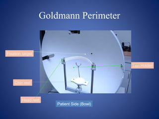
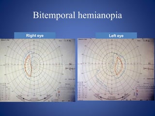
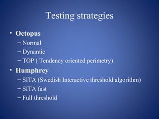

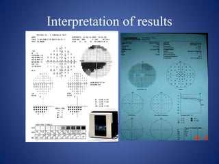

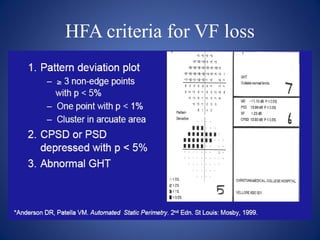


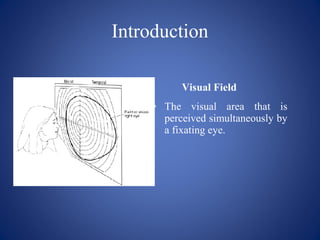
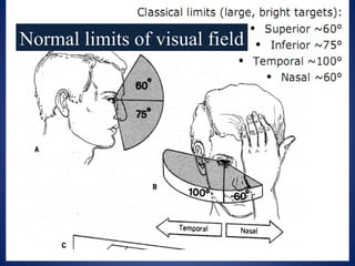
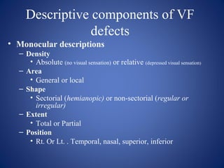
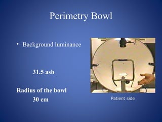
This document provides an overview of visual field testing and interpretation. It begins with definitions of key visual field terminology. It then discusses the history of visual field testing and describes common testing methods like kinetic and static perimetry. Goldmann perimetry and automated perimetry are explained in detail. The document reviews how to interpret visual field results, including expected normal limits and descriptions of common visual field defects. It provides guidelines for visual field testing and plotting isopters. Overall, the document serves as a comprehensive guide to visual field assessment.


![ONFH[AVN HIP] -TRIPLE REGIME -A NOVAL SURGICAL CONCEPT .pptx](https://cdn.slidesharecdn.com/ss_thumbnails/onfhavnhip2026koaconcalicutdrgokuldevdrmashraf-260210064517-213ec005-thumbnail.jpg?width=640&height=640&fit=bounds)


