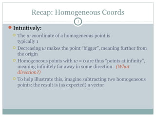
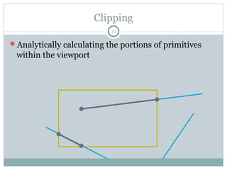
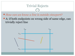
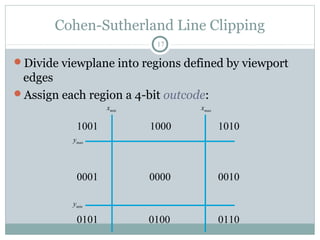
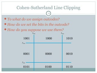
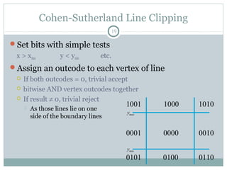
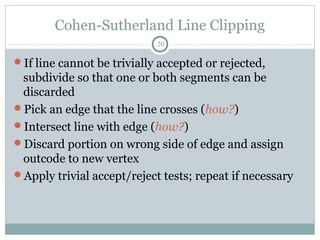
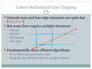
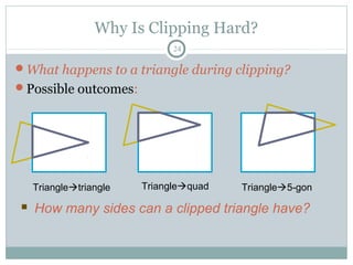
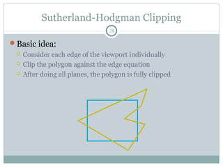
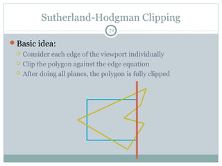
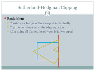
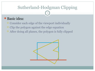
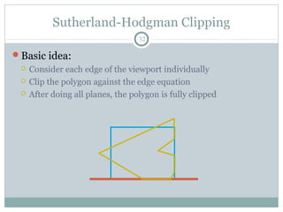
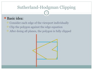
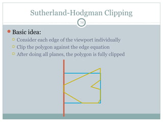
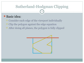
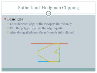
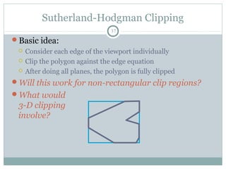
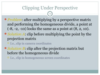
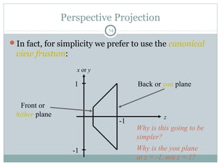
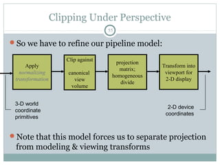
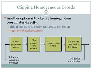
Clipping is a technique used to remove portions of lines, polygons, and other primitives that lie outside the visible viewing area or viewport. There are several common clipping algorithms. Cohen-Sutherland line clipping uses bit codes to quickly determine if a line segment can be fully accepted or rejected for clipping. Sutherland-Hodgman polygon clipping considers each viewport edge individually, clips the polygon against that edge plane, and generates a new clipped polygon. Perspective projection transforms 3D objects to 2D screen coordinates, and clipping must account for objects behind the viewer; this can be done by clipping in camera coordinates before perspective projection or in homogeneous screen coordinates after projection.

1. PRESENTED BY
BARANITHARAN
COMPUTER SCIENCE AND ENGINEERING
KINGS COLLEGE OF ENGINEERING
Clipping

2. Outline
2
Review
Clipping Basics
Cohen-Sutherland Line Clipping
Clipping Polygons
Sutherland-Hodgman Clipping
Perspective Clipping

3. Recap: Homogeneous Coords
3
Intuitively:
 The w coordinate of a homogeneous point is
typically 1
 Decreasing w makes the point “bigger”, meaning further from
the origin
 Homogeneous points with w = 0 are thus “points at infinity”,
meaning infinitely far away in some direction. (What
direction?)
 To help illustrate this, imagine subtracting two homogeneous
points: the result is (as expected) a vector

4. Recap: Perspective Projection
4
When we do 3-D graphics, we think of the
screen as a 2-D window onto the 3-D world:
How tall should
this bunny be?

5. Recap: Perspective Projection
5
The geometry of the situation:
Desired
result:
P (x, y, z)X
Z
View
plane
d
(0,0,0) x’ = ?
' , ' ,
d x x d y y
x y z d
z z d z z d
× ×
= = = = =

6. Recap: Perspective Projection Matrix
6
Example:
Or, in 3-D coordinates:
























=












10100
0100
0010
0001
z
y
x
ddz
z
y
x






d
dz
y
dz
x
,,

7. Recap: OpenGL’s Persp. Proj. Matrix
7
OpenGL’s gluPerspective() command generates
a slightly more complicated matrix:
 Can you figure out what this matrix does?






=


















−








−
××








−
+
2
cotwhere
0100
2
00
000
000
y
farnear
nearfar
farnear
nearfar
fov
f
ZZ
ZZ
ZZ
ZΖ
f
aspect
f

8. Projection Matrices
8
Now that we can express perspective foreshortening
as a matrix, we can composite it onto our other
matrices with the usual matrix multiplication
End result: can create a single matrix encapsulating
modeling, viewing, and projection transforms
 Though you will recall that in practice OpenGL separates the
modelview from projection matrix (why?)

9. Outline
9
Review
Clipping Basics
Cohen-Sutherland Line Clipping
Clipping Polygons
Sutherland-Hodgman Clipping
Perspective Clipping

10. Next Topic: Clipping
10
We’ve been assuming that all primitives (lines,
triangles, polygons) lie entirely within the viewport
In general, this assumption will not hold

11. Clipping
11
Analytically calculating the portions of primitives
within the viewport

12. Why Clip?
12
Bad idea to rasterize outside of framebuffer bounds
Also, don’t waste time scan converting pixels outside
window

13. Clipping
13
The naïve approach to clipping lines:
for each line segment
for each edge of viewport
find intersection points
pick “nearest” point
if anything is left, draw it
What do we mean by “nearest”?
How can we optimize this?

14. Trivial Accepts
14
Big optimization: trivial accept/rejects
How can we quickly determine whether a line
segment is entirely inside the viewport?
A: test both endpoints.
xmin xmax
ymax
ymin

15. Trivial Rejects
15
How can we know a line is outside viewport?
A: if both endpoints on wrong side of same edge, can
trivially reject line
xmin xmax
ymax
ymin

16. Outline
16
Review
Clipping Basics
Cohen-Sutherland Line Clipping
Clipping Polygons
Sutherland-Hodgman Clipping
Perspective Clipping

17. Cohen-Sutherland Line Clipping
17
Divide viewplane into regions defined by viewport
edges
Assign each region a 4-bit outcode:
0000 00100001
1001
0101 0100
1000 1010
0110
xmin xmax
ymax
ymin

18. Cohen-Sutherland Line Clipping
18
To what do we assign outcodes?
How do we set the bits in the outcode?
How do you suppose we use them?
xmin xmax
0000 00100001
1001
0101 0100
1000 1010
0110
ymax
ymin

19. Cohen-Sutherland Line Clipping
19
Set bits with simple tests
x > xmax y < ymin etc.
Assign an outcode to each vertex of line
 If both outcodes = 0, trivial accept
 bitwise AND vertex outcodes together
 If result ≠ 0, trivial reject
 As those lines lie on one
side of the boundary lines
0000 00100001
1001
0101 0100
1000 1010
0110
ymax
ymin

20. Cohen-Sutherland Line Clipping
20
If line cannot be trivially accepted or rejected,
subdivide so that one or both segments can be
discarded
Pick an edge that the line crosses (how?)
Intersect line with edge (how?)
Discard portion on wrong side of edge and assign
outcode to new vertex
Apply trivial accept/reject tests; repeat if necessary

21. Cohen-Sutherland Line Clipping
21
Outcode tests and line-edge intersects are quite fast
(how fast?)
But some lines require multiple iterations:
 Clip top
 Clip left
 Clip bottom
 Clip right
Fundamentally more efficient algorithms:
 Cyrus-Beck uses parametric lines
 Liang-Barsky optimizes this for upright volumes

22. Outline
22
Review
Clipping Basics
Cohen-Sutherland Line Clipping
Clipping Polygons
Sutherland-Hodgman Clipping
Perspective Clipping

23. Clipping Polygons
23
We know how to clip a single line segment
 How about a polygon in 2D?
 How about in 3D?
Clipping polygons is more complex than clipping the
individual lines
 Input: polygon
 Output: polygon, or nothing
When can we trivially accept/reject a polygon as
opposed to the line segments that make up the
polygon?

24. Why Is Clipping Hard?
24
What happens to a triangle during clipping?
Possible outcomes:
Triangletriangle Trianglequad Triangle5-gon
 How many sides can a clipped triangle have?

25. Why Is Clipping Hard?
25
A really tough case:

26. Why Is Clipping Hard?
26
A really tough case:
concave polygonmultiple polygons

27. Outline
27
Review
Clipping Basics
Cohen-Sutherland Line Clipping
Clipping Polygons
Sutherland-Hodgman Clipping
Perspective Clipping

28. Sutherland-Hodgman Clipping
28
Basic idea:
 Consider each edge of the viewport individually
 Clip the polygon against the edge equation
 After doing all planes, the polygon is fully clipped

29. Sutherland-Hodgman Clipping
29
Basic idea:
 Consider each edge of the viewport individually
 Clip the polygon against the edge equation
 After doing all planes, the polygon is fully clipped

30. Sutherland-Hodgman Clipping
30
Basic idea:
 Consider each edge of the viewport individually
 Clip the polygon against the edge equation
 After doing all planes, the polygon is fully clipped

31. Sutherland-Hodgman Clipping
31
Basic idea:
 Consider each edge of the viewport individually
 Clip the polygon against the edge equation
 After doing all planes, the polygon is fully clipped

32. Sutherland-Hodgman Clipping
32
Basic idea:
 Consider each edge of the viewport individually
 Clip the polygon against the edge equation
 After doing all planes, the polygon is fully clipped

33. Sutherland-Hodgman Clipping
33
Basic idea:
 Consider each edge of the viewport individually
 Clip the polygon against the edge equation
 After doing all planes, the polygon is fully clipped

34. Sutherland-Hodgman Clipping
34
Basic idea:
 Consider each edge of the viewport individually
 Clip the polygon against the edge equation
 After doing all planes, the polygon is fully clipped

35. Sutherland-Hodgman Clipping
35
Basic idea:
 Consider each edge of the viewport individually
 Clip the polygon against the edge equation
 After doing all planes, the polygon is fully clipped

36. Sutherland-Hodgman Clipping
36
Basic idea:
 Consider each edge of the viewport individually
 Clip the polygon against the edge equation
 After doing all planes, the polygon is fully clipped

37. Sutherland-Hodgman Clipping
37
Basic idea:
 Consider each edge of the viewport individually
 Clip the polygon against the edge equation
 After doing all planes, the polygon is fully clipped
Will this work for non-rectangular clip regions?
What would
3-D clipping
involve?

38. Sutherland-Hodgman Clipping
38
Input/output for algorithm:
 Input: list of polygon vertices in order
 Output: list of clipped polygon vertices consisting of old
vertices (maybe) and new vertices (maybe)
Note: this is exactly what we expect from the
clipping operation against each edge
This algorithm generalizes to 3-D
 Show movie…

39. Sutherland-Hodgman Clipping
39
We need to be able to create clipped polygons from
the original polygons
Sutherland-Hodgman basic routine:
 Go around polygon one vertex at a time
 Current vertex has position p
 Previous vertex had position s, and it has been added to the
output if appropriate

40. Sutherland-Hodgman Clipping
40
Edge from s to p takes one of four cases:
(Purple line can be a line or a plane)
inside outside
s
p
p output
inside outside
s
p
no output
inside outside
s
p
i output
inside outside
sp
i output
p output

41. Sutherland-Hodgman Clipping
41
Four cases:
 s inside plane and p inside plane
 Add p to output
 Note: s has already been added
 s inside plane and p outside plane
 Find intersection point i
 Add i to output
 s outside plane and p outside plane
 Add nothing
 s outside plane and p inside plane
 Find intersection point i
 Add i to output, followed by p

42. Point-to-Plane test
42
A very general test to determine if a point p is
“inside” a plane P, defined by q and n:
(p - q) • n < 0: p inside P
(p - q) • n = 0: p on P
(p - q) • n > 0: p outside P
P
n
p
q
P
n
p
q
P
n
p
q

43. Point-to-Plane Test
43
Dot product is relatively expensive
 3 multiplies
 5 additions
 1 comparison (to 0, in this case)
Think about how you might optimize or special-case
this

44. Finding Line-Plane Intersections
44
Use parametric definition of edge:
E(t) = s + t(p - s)
 If t = 0 then E(t) = s
 If t = 1 then E(t) = p
 Otherwise, E(t) is part way from s to p

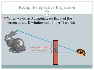
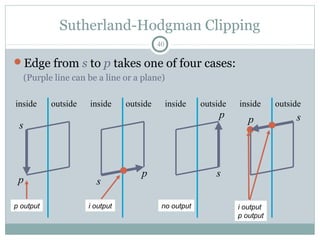
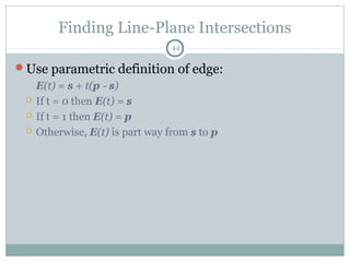
45. Finding Line-Plane Intersections
45
Edge intersects plane P where E(t) is on P
 q is a point on P
 n is normal to P
(E(t) - q) • n = 0
(s + t(p - s) - q) • n = 0
t = [(q - s) • n] / [(p - s) • n]
 The intersection point i = E(t) for this value of t

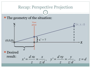
46. Line-Plane Intersections
46
Note that the length of n doesn’t affect result:
t = [(q - s) • n] / [(p - s) • n]
Again, lots of opportunity for optimization

47. Outline
47
Review
Clipping Basics
Cohen-Sutherland Line Clipping
Clipping Polygons
Sutherland-Hodgman Clipping
Perspective Clipping

48. 3-D Clipping
48
Before actually drawing on the screen, we have to
clip (Why?)
Can we transform to screen coordinates first, then
clip in 2D?
 Correctness: shouldn’t draw objects behind viewer
 What will an object with negative z coordinates do in our
perspective matrix?

49. Recap: Perspective Projection Matrix
49
Example:
Or, in 3-D coordinates:
Multiplying by the projection matrix gets us the 3-D
coordinates
The act of dividing x and y by z/d is called the
homogeneous divide
























=












10100
0100
0010
0001
z
y
x
ddz
z
y
x






d
dz
y
dz
x
,,

50. Clipping Under Perspective
50
Problem: after multiplying by a perspective matrix
and performing the homogeneous divide, a point at
(-8, -2, -10) looks the same as a point at (8, 2, 10).
Solution A: clip before multiplying the point by the
projection matrix
 I.e., clip in camera coordinates
Solution B: clip after the projection matrix but
before the homogeneous divide
 I.e., clip in homogeneous screen coordinates

51. Clipping Under Perspective
51
We will talk first about solution A:
Clip against
view volume
Apply projection
matrix and
homogeneous
divide
Transform into
viewport for
2-D display
3-D world
coordinate
primitives
Clipped world
coordinates
2-D device
coordinates
Canonical screen
coordinates

52. Recap: Perspective Projection
52
The typical view volume is a frustum or truncated
pyramid
x or y
z

53. Perspective Projection
53
The viewing frustum consists of six planes
The Sutherland-Hodgeman algorithm (clipping
polygons to a region one plane at a time) generalizes
to 3-D
 Clip polygons against six planes of view frustum
 So what’s the problem?
The problem: clipping a line segment to an arbitrary
plane is relatively expensive
 Dot products and such

54. Perspective Projection
54
In fact, for simplicity we prefer to use the canonical
view frustum:
x or y
1
-1
z
-1
Front or
hither plane
Back or yon plane
Why is this going to be
simpler?
Why is the yon plane
at z = -1, not z = 1?

55. Clipping Under Perspective
55
So we have to refine our pipeline model:
Note that this model forces us to separate projection
from modeling & viewing transforms
Apply
normalizing
transformation
projection
matrix;
homogeneous
divide
Transform into
viewport for
2-D display
3-D world
coordinate
primitives
2-D device
coordinates
Clip against
canonical
view
volume

56. Clipping Homogeneous Coords
56
Another option is to clip the homogeneous
coordinates directly.
 This allows us to clip after perspective projection:
 What are the advantages?
Clip
against
view
volume
Apply
projection
matrix
Transform into
viewport for
2-D display
3-D world
coordinate
primitives
2-D device
coordinates
Homogeneous
divide

57. Clipping Homogeneous Coords
57
Other advantages:
 Can transform the canonical view volume for perspective
projections to the canonical view volume for parallel
projections
 Clip in the latter (only works in homogeneous coords)
 Allows an optimized (hardware) implementation
 Some primitives will have w ≠ 1
 For example, polygons that result from tesselating splines
 Without clipping in homogeneous coords, must perform divide
twice on such primitives

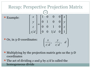
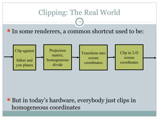
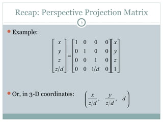
58. Clipping Homogeneous Coords
58
So how do we clip homogeneous coordinates?
Briefly, thus:
 Remember that we have applied a transform to normalized
device coordinates
 x, y  [-1, 1]
 z  [0, 1]
 When clipping to (say) right side of the screen (x = 1), instead
clip to (x = w)
Can find details in book or on web

59. Clipping: The Real World
59
In some renderers, a common shortcut used to be:
But in today’s hardware, everybody just clips in
homogeneous coordinates
Projection
matrix;
homogeneous
divide
Clip in 2-D
screen
coordinates
Clip against
hither and
yon planes
Transform into
screen
coordinates