Knapsack problem and Memory Function

KNAPSACK PROBLEM AND MEMORY
FUNCTION
PREPARED BY
M. Baranitharan
Kings College of Engineering

Given some items, pack the knapsack to get
the maximum total value. Each item has some
weight and some value. Total weight that we can
carry is no more than some fixed number W.
So we must consider weights of items as well as
their values.
Item # Weight Value
1 1 8
2 3 6
3 5 5

There are two versions of the problem:
1. “0-1 knapsack problem”
 Items are indivisible; you either take an item or not.
Some special instances can be solved with dynamic
programming
1. “Fractional knapsack problem”
 Items are divisible: you can take any fraction of an
item

 Given a knapsack with maximum capacity W, and
a set S consisting of n items
 Each item i has some weight wi and benefit value
bi (all wi and W are integer values)
 Problem: How to pack the knapsack to achieve
maximum total value of packed items?

 Problem, in other words, is to find
∑∑ ∈∈
≤
Ti
i
Ti
i Wwb subject tomax
The problem is called a “0-1” problem,
because each item must be entirely
accepted or rejected.

Let’s first solve this problem with a
straightforward algorithm
 Since there are n items, there are 2n
possible
combinations of items.
 We go through all combinations and find the
one with maximum value and with total weight
less or equal to W
 Running time will be O(2n
)

 We can do better with an algorithm based on
dynamic programming
 We need to carefully identify the subproblems

 We can do better with an algorithm based on
dynamic programming
 We need to carefully identify the subproblems
Let’s try this:
If items are labeled 1..n, then a subproblem
would be to find an optimal solution for
Sk = {items labeled 1, 2, .. k}

If items are labeled 1..n, then a subproblem
would be to find an optimal solution for Sk =
{items labeled 1, 2, .. k}
 This is a reasonable subproblem definition.
 The question is: can we describe the final
solution (Sn ) in terms of subproblems (Sk)?
 Unfortunately, we can’t do that.

Max weight: W = 20
For S4:
Total weight: 14
Maximum benefit: 20
w1 =2
b1 =3
w2 =4
b2 =5
w3 =5
b3 =8
w4 =3
b4 =4 wi bi
10
85
54
43
32
Weight Benefit
9
Item
#
4
3
2
1
5
S4
S5
w1 =2
b1 =3
w2 =4
b2 =5
w3 =5
b3 =8
w5 =9
b5 =10
For S5:
Total weight: 20
Maximum benefit: 26
Solution for S4 is
not part of the
solution for S !!!
?

 As we have seen, the solution for S4 is not part of
the solution for S5
 So our definition of a subproblem is flawed and we
need another one!

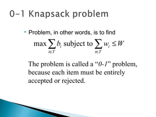
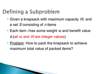
 Let’s add another parameter: w, which will
represent the maximum weight for each subset of
items
 The subproblem then will be to compute V[k,w],
i.e., to find an optimal solution for Sk = {items
labeled 1, 2, .. k} in a knapsack of size w

 The subproblem will then be to compute V[k,w],
i.e., to find an optimal solution for Sk = {items
labeled 1, 2, .. k} in a knapsack of size w
 Assuming knowing V[i, j], where i=0,1, 2, … k-1,
j=0,1,2, …w, how to derive V[k,w]?

It means, that the best subset of Sk that has total
weight w is:
1) the best subset of Sk-1 that has total weight ≤ w, or
2) the best subset of Sk-1 that has total weight ≤ w-wk plus
the item k



+−−−
>−
=
else}],1[],,1[max{
if],1[
],[
kk
k
bwwkVwkV
wwwkV
wkV
Recursive formula for subproblems:

 The best subset of Sk that has the total weight ≤ w,
either contains item k or not.
 First case: wk>w. Item k can’t be part of the solution,
since if it was, the total weight would be > w, which is
unacceptable.
 Second case: wk ≤ w. Then the item k can be in the
solution, and we choose the case with greater value.



+−−−
>−
=
else}],1[],,1[max{
if],1[
],[
kk
k
bwwkVwkV
wwwkV
wkV

for w = 0 to W
V[0,w] = 0
for i = 1 to n
V[i,0] = 0
for i = 1 to n
for w = 0 to W
if wi <= w // item i can be part of the solution
if bi + V[i-1,w-wi] > V[i-1,w]
V[i,w] = bi + V[i-1,w- wi]
else
V[i,w] = V[i-1,w]
else V[i,w] = V[i-1,w] // wi > w

for w = 0 to W
V[0,w] = 0
for i = 1 to n
V[i,0] = 0
for i = 1 to n
for w = 0 to W
< the rest of the code >
What is the running time of this
algorithm?
O(W)
O(W)
Repeat n times
O(n*W)
Remember that the brute-force algorithm
takes O(2n
)

Let’s run our algorithm on the
following data:
n = 4 (# of elements)
W = 5 (max weight)
Elements (weight, benefit):
(2,3), (3,4), (4,5), (5,6)

for w = 0 to W
V[0,w] = 0
0 0 0 0 000
1
2
3
4 50 1 2 3
4
iW

for i = 1 to n
V[i,0] = 0
0
0
0
0
0 0 0 0 000
1
2
3
4 50 1 2 3
4
iW

V[i,w] = bi + V[i-1,w- wi]
else
V[i,w] = V[i-1,w]
0
Items:
1: (2,3)
2: (3,4)
3: (4,5)
4: (5,6)
0
i=1
bi=3
wi=2
w=1
w-wi =-1
0 0 0 0 000
1
2
3
4 50 1 2 3
4
iW
0
0
0

Items:
1: (2,3)
2: (3,4)
3: (4,5)
4: (5,6)
300
0
0
0
0 0 0 0 000
1
2
3
4 50 1 2 3
4
iW
i=1
bi=3
wi=2
w=4
w-wi =2
V[i,w] = bi + V[i-1,w- wi]
else
V[i,w] = V[i-1,w]
3 3

Items:
1: (2,3)
2: (3,4)
3: (4,5)
4: (5,6)
300
0
0
0
0 0 0 0 000
1
2
3
4 50 1 2 3
4
iW
i=1
bi=3
wi=2
w=5
w-wi =3
V[i,w] = bi + V[i-1,w- wi]
else
V[i,w] = V[i-1,w]
3 3 3

Items:
1: (2,3)
2: (3,4)
3: (4,5)
4: (5,6)
00
0
0
0
0 0 0 0 000
1
2
3
4 50 1 2 3
4
iW
i=2
bi=4
wi=3
w=2
w-wi =-1
3 3 3 3
3
V[i,w] = bi + V[i-1,w- wi]
else
V[i,w] = V[i-1,w]
0

Items:
1: (2,3)
2: (3,4)
3: (4,5)
4: (5,6)
00
0
0
0
0 0 0 0 000
1
2
3
4 50 1 2 3
4
iW
i=2
bi=4
wi=3
w=3
w-wi =0
3 3 3 3
0
V[i,w] = bi + V[i-1,w- wi]
else
V[i,w] = V[i-1,w]
43

Items:
1: (2,3)
2: (3,4)
3: (4,5)
4: (5,6)
00
0
0
0
0 0 0 0 000
1
2
3
4 50 1 2 3
4
iW
i=3
bi=5
wi=4
w= 1..3
3 3 3 3
0 3 4 4
V[i,w] = bi + V[i-1,w- wi]
else
V[i,w] = V[i-1,w]
7
3 40

Items:
1: (2,3)
2: (3,4)
3: (4,5)
4: (5,6)
00
0
0
0
0 0 0 0 000
1
2
3
4 50 1 2 3
4
iW
i=4
bi=6
wi=5
w= 1..4
3 3 3 3
0 3 4 4
V[i,w] = bi + V[i-1,w- wi]
else
V[i,w] = V[i-1,w]
7
3 40
70 3 4 5
5

Items:
1: (2,3)
2: (3,4)
3: (4,5)
4: (5,6)
00
0
0
0
0 0 0 0 000
1
2
3
4 50 1 2 3
4
iW
i=4
bi=6
wi=5
w= 5
w- wi=0
3 3 3 3
0 3 4 4 7
0 3 4
V[i,w] = bi + V[i-1,w- wi]
else
V[i,w] = V[i-1,w]
5
7
7
0 3 4 5

 This algorithm only finds the max possible value
that can be carried in the knapsack
◦ i.e., the value in V[n,W]
 To know the items that make this maximum value,
an addition to this algorithm is necessary

 All of the information we need is in the table.
 V[n,W] is the maximal value of items that can be
placed in the Knapsack.
 Let i=n and k=W
if V[i,k] ≠ V[i−1,k] then
mark the ith
item as in the knapsack
i = i−1, k = k-wi
else
i = i−1 // Assume the ith
item is not in the knapsack
// Could it be in the optimally packed
knapsack?

 Goal:
◦ Solve only subproblems that are necessary and solve it only once
 Memorization is another way to deal with overlapping subproblems
in dynamic programming
 With memorization, we implement the algorithm recursively:
◦ If we encounter a new subproblem, we compute and store the solution.
◦ If we encounter a subproblem we have seen, we look up the answer
 Most useful when the algorithm is easiest to implement recursively
◦ Especially if we do not need solutions to all subproblems.

for i = 1 to n
for w = 1 to W
V[i,w] = -1
for w = 0 to W
V[0,w] = 0
for i = 1 to n
V[i,0] = 0
MFKnapsack(i, w)
if V[i,w] < 0
if w < wi
value = MFKnapsack(i-1, w)
else
value = max(MFKnapsack(i-1, w),
bi + MFKnapsack(i-1, w-wi))
V[i,w] = value
return V[i,w]

 Dynamic programming is a useful technique of
solving certain kind of problems
 When the solution can be recursively described
in terms of partial solutions, we can store these
partial solutions and re-use them as necessary
(memorization)
 Running time of dynamic programming
algorithm vs. naïve algorithm:
◦ 0-1 Knapsack problem: O(W*n) vs. O(2n
)

Design and Analysis of Algorithms - Chapter 8 36

Knapsack problem and Memory Function

Recommended

Recommended

More Related Content

What's hot

What's hot (20)

Similar to Knapsack problem and Memory Function

Similar to Knapsack problem and Memory Function (20)

More from Barani Tharan

More from Barani Tharan (14)

Recently uploaded

Recently uploaded (20)

Knapsack problem and Memory Function