Downloaded 252 times


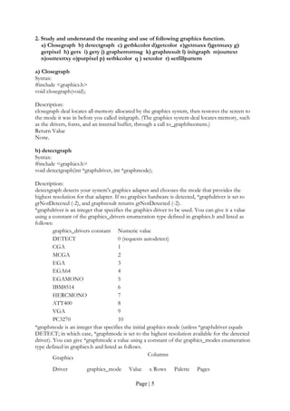


![Page | 22
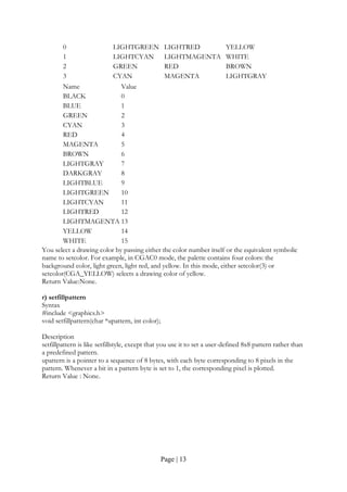
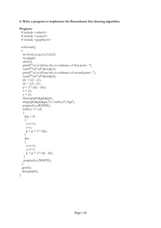
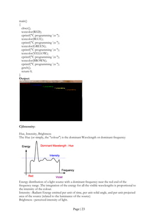
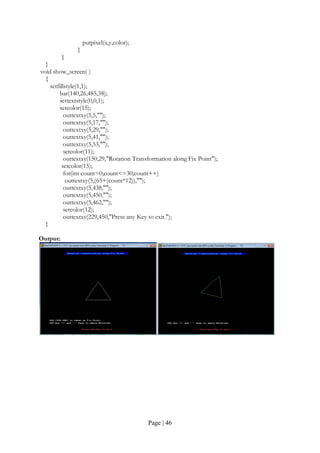
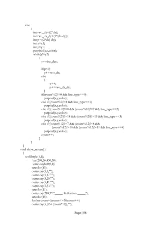
8. Write a program to show the following attribute of output primitives.
A) Line style B) Color C) Intensity
A) Line styles
Program:
#include <graphics.h>
#include <stdlib.h>
#include <string.h>
#include <stdio.h>
#include <conio.h>
void main()
{
int gd=DETECT,gm;
int s;
char *lname[]={"SOLID LINE","DOTTED LINE","CENTER LINE",
"DASHED LINE","USERBIT LINE"};
initgraph(&gd,&gm,"c:turboc3bgi");
clrscr();
cleardevice();
printf("Line styles:");
for (s=0;s<5;s++)
{
setlinestyle(s,1,3);
line(100,30+s*50,250,250+s*50);
outtextxy(255,250+s*50,lname[s]);
}
getch();
closegraph();
}
Output:
B)Color
Program:
#include<stdio.h>
#include<conio.h>](https://image.slidesharecdn.com/cgfile-140420070604-phpapp01/85/Computer-Graphics-Programes-22-320.jpg)
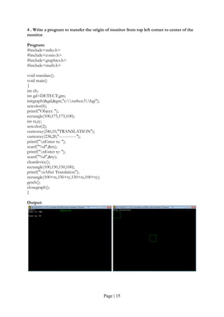
![Page | 27
y_1=0;
x_2=0;
y_2=0;
}
LineCoordinates(const float x1,const float y1, const float x2,const float y2)
{
x_1=x1;
y_1=y1;
x_2=x2;
y_2=y2;
}
};
void show_screen( );
void Fill_polygon(const int,const int [],const int);
void insertEdge(Edge *,Edge *);
void makeEdgeRec(const PointCoordinates,const PointCoordinates, const int,Edge *,Edge *[]);
void buildEdgeList(const int,const PointCoordinates [],Edge *[]);
void buildActiveList(const int,Edge *,Edge *[]);
void fillScan(const int,const Edge *,const int);
void deleteAfter(Edge []);
void updateActiveList(const int,Edge []);
void resortActiveList(Edge []);
const int yNext(const int,const int,const PointCoordinates []);
void Polygon(const int,const int []);
void Line(const int,const int,const int,const int);
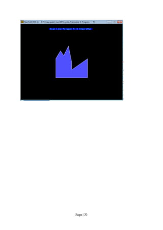
int main( )
{
int driver=VGA;
int mode=VGAHI;
initgraph(&driver,&mode,"..Bgi");
show_screen( );
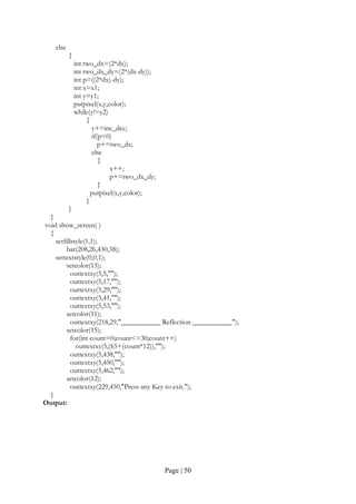
int n=10;
int polygon_points[20]={ 220,340 , 220,220 , 250,170 , 270,200 , 300,140 , 320,240 , 320,290
, 420,220 ,420,340 , 220,340 };
setcolor(15);
Polygon(10,polygon_points);
Fill_polygon(n,polygon_points,9);
getch( );
return 0;
}
void Fill_polygon(const int n,const int ppts[],const int fill_color)
{
Edge *edges[480];
Edge *active;
PointCoordinates *pts=new PointCoordinates[n];
for(int count_1=0;count_1<n;count_1++)
{
pts[count_1].x=(ppts[(count_1*2)]);
pts[count_1].y=(ppts[((count_1*2)+1)]);
}
for(int count_2=0;count_2<640;count_2++)](https://image.slidesharecdn.com/cgfile-140420070604-phpapp01/85/Computer-Graphics-Programes-27-320.jpg)
![Page | 28
{
edges[count_2]=new Edge;
edges[count_2]->next=NULL;
}
buildEdgeList(n,pts,edges);
active=new Edge;
active->next=NULL;
for(int count_3=0;count_3<480;count_3++)
{
buildActiveList(count_3,active,edges);
if(active->next)
{
fillScan(count_3,active,fill_color);
updateActiveList(count_3,active);
resortActiveList(active);
}
}
Polygon(n,ppts);
delete pts;
}
const int yNext(const int k,const int cnt,const PointCoordinates pts[])
{
int j;
if((k+1)>(cnt-1))
j=0;
else
j=(k+1);
while(pts[k].y==pts[j].y)
{
if((j+1)>(cnt-1))
j=0;
else
j++;
}
return (pts[j].y);
}
void insertEdge(Edge *list,Edge *edge)
{
Edge *p;
Edge *q=list;
p=q->next;
while(p!=NULL)
{
if(edge->xIntersect<p->xIntersect)
p=NULL;
else
{
q=p;
p=p->next;
}](https://image.slidesharecdn.com/cgfile-140420070604-phpapp01/85/Computer-Graphics-Programes-28-320.jpg)
![Page | 29
edge->next=q->next;
q->next=edge;
}
void makeEdgeRec(const PointCoordinates lower,const PointCoordinates upper,
const int yComp,Edge *edge,Edge *edges[])
{
edge->dxPerScan=((upper.x-lower.x)/(upper.y-lower.y));
edge->xIntersect=lower.x;
if(upper.y<yComp)
edge->yUpper=(upper.y-1);
else
edge->yUpper=upper.y;
insertEdge(edges[lower.y],edge);
}
void buildEdgeList(const int cnt,const PointCoordinates pts[],Edge *edges[])
{
Edge *edge;
PointCoordinates v1;
PointCoordinates v2;
int yPrev=(pts[cnt-2].y);
v1.x=pts[cnt-1].x;
v1.y=pts[cnt-1].y;
for(int count=0;count<cnt;count++)
{
v2=pts[count];
if(v1.y!=v2.y)
{
edge=new Edge;
if(v1.y<v2.y)
makeEdgeRec(v1,v2,yNext(count,cnt,pts),edge,edges);
else
makeEdgeRec(v2,v1,yPrev,edge,edges);
}
yPrev=v1.y;
v1=v2;
}
}
void buildActiveList(const int scan,Edge *active,Edge *edges[])
{
Edge *p;
Edge *q;
p=edges[scan]->next;
while(p)
{
q=p->next;
insertEdge(active,p);
p=q;
}
}
void fillScan(const int scan,const Edge *active,const int fill_color)
{](https://image.slidesharecdn.com/cgfile-140420070604-phpapp01/85/Computer-Graphics-Programes-29-320.jpg)
![Page | 31
}
void Polygon(const int n,const int coordinates[])
{
if(n>=2)
{
Line(coordinates[0],coordinates[1], coordinates[2],coordinates[3]);
for(int count=1;count<(n-1);count++)
Line(coordinates[(count*2)],coordinates[((count*2)+1)], coordinates[((count+1)*2)],
coordinates[(((count+1)*2)+1)]);
}
}
void Line(const int x_1,const int y_1,const int x_2,const int y_2)
{
int color=getcolor( );
int x1=x_1;
int y1=y_1;
int x2=x_2;
int y2=y_2;
if(x_1>x_2)
{
x1=x_2;
y1=y_2;
x2=x_1;
y2=y_1;
}
int dx=abs(x2-x1);
int dy=abs(y2-y1);
int inc_dec=((y2>=y1)?1:-1);
if(dx>dy)
{
int two_dy=(2*dy);
int two_dy_dx=(2*(dy-dx));
int p=((2*dy)-dx);
int x=x1;
int y=y1;
putpixel(x,y,color);
while(x<x2)
{
x++;
if(p<0)
p+=two_dy;
else
{
y+=inc_dec;
p+=two_dy_dx;
}
putpixel(x,y,color);
}
}
else](https://image.slidesharecdn.com/cgfile-140420070604-phpapp01/85/Computer-Graphics-Programes-31-320.jpg)
![Page | 34
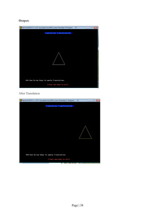
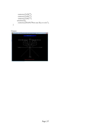
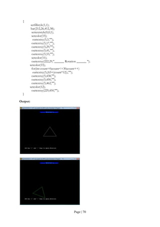
10. Write a program to perform translation of two dimensional objects.
Program:
# include <iostream.h>
# include <graphics.h>
# include <conio.h>
# include <math.h
void show_screen( );
void apply_translation(const int,int [],const int,const int);
void multiply_matrices(const int[3],const int[3][3],int[3]);
void Polygon(const int,const int []);
void Line(const int,const int,const int,const int);
int main( )
{
int driver=VGA;
int mode=VGAHI;
initgraph(&driver,&mode,"..Bgi");
show_screen( );
int polygon_points[8]={ 270,290, 320,190, 370,290, 270,290 };
setcolor(15);
Polygon(4,polygon_points);
setcolor(15);
settextstyle(0,0,1);
outtextxy(50,415,"*** Use Arrow Keys to apply Translation.");
int key_code_1=0;
int key_code_2=0;
char Key_1=NULL;
char Key_2=NULL;
do
{
Key_1=NULL;
Key_2=NULL;
key_code_1=0;
key_code_2=0;
Key_1=getch( );
key_code_1=int(Key_1);
if(key_code_1==0)
{
Key_2=getch( );
key_code_2=int(Key_2);
}
if(key_code_1==27)
break;
else if(key_code_1==0)
{
if(key_code_2==72)
{
setfillstyle(1,0);
bar(40,70,600,410);
apply_translation(4,polygon_points,0,-25);
setcolor(10);](https://image.slidesharecdn.com/cgfile-140420070604-phpapp01/85/Computer-Graphics-Programes-34-320.jpg)
![Page | 35
Polygon(4,polygon_points);
}
else if(key_code_2==75)
{
setfillstyle(1,0);
bar(40,70,600,410);
apply_translation(4,polygon_points,-25,0);
setcolor(12);
Polygon(4,polygon_points);
}
else if(key_code_2==77)
{
setfillstyle(1,0);
bar(40,70,600,410);
apply_translation(4,polygon_points,25,0);
setcolor(14);
Polygon(4,polygon_points);
}
else if(key_code_2==80)
{
setfillstyle(1,0);
bar(40,70,600,410);
apply_translation(4,polygon_points,0,25);
setcolor(9);
Polygon(4,polygon_points);
}
}
}
while(1);
return 0;
}
void apply_translation(const int n,int coordinates[],const int Tx,const int Ty)
{
for(int count_1=0;count_1<n;count_1++)
{
int matrix_a[3]={coordinates[(count_1*2)], coordinates[((count_1*2)+1)],1};
int matrix_b[3][3]={ {1,0,0} , {0,1,0} ,{ Tx,Ty,1} };
int matrix_c[3]={0};
multiply_matrices(matrix_a,matrix_b,matrix_c);
coordinates[(count_1*2)]=matrix_c[0];
coordinates[((count_1*2)+1)]=matrix_c[1];
}
}
void multiply_matrices(const int matrix_1[3],const int matrix_2[3][3],int matrix_3[3])
{
for(int count_1=0;count_1<3;count_1++)
{
for(int count_2=0;count_2<3;count_2++)
matrix_3[count_1]+= (matrix_1[count_2]*matrix_2[count_2][count_1]);
}
}](https://image.slidesharecdn.com/cgfile-140420070604-phpapp01/85/Computer-Graphics-Programes-35-320.jpg)
![Page | 36
void Polygon(const int n,const int coordinates[])
{
if(n>=2)
{
Line(coordinates[0],coordinates[1],coordinates[2],coordinates[3]);
for(int count=1;count<(n-1);count+
Line(coordinates[(count*2)],coordinates[((count*2)+1)],coordinates[((count+1)*2)],
coordinates[(((count+1)*2)+1)]);
}
}
void Line(const int x_1,const int y_1,const int x_2,const int y_2)
{
int color=getcolor( );
int x1=x_1;
int y1=y_1;
int x2=x_2;
int y2=y_2;
if(x_1>x_2)
{
x1=x_2;
y1=y_2;
x2=x_1;
y2=y_1;
}
int dx=abs(x2-x1);
int dy=abs(y2-y1);
int inc_dec=((y2>=y1)?1:-1);
if(dx>dy)
{
int two_dy=(2*dy);
int two_dy_dx=(2*(dy-dx));
int p=((2*dy)-dx);
int x=x1;
int y=y1;
putpixel(x,y,color);
while(x<x2)
{
x++;
if(p<0)
p+=two_dy;
else
{
y+=inc_dec;
p+=two_dy_dx;
}
putpixel(x,y,color);
}
}
else
{
int two_dx=(2*dx);](https://image.slidesharecdn.com/cgfile-140420070604-phpapp01/85/Computer-Graphics-Programes-36-320.jpg)
![Page | 39
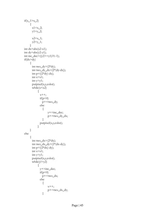
11. Write a program to perform scaling of two dimensional objects.
A) About the origin B) About fixed point
Program:
# include <iostream.h>
# include <graphics.h>
# include <conio.h>
# include <math.h>
void show_screen( );
void apply_fixed_point_scaling(const int,int [],const float, const float,const int,const int);
void multiply_matrices(const float[3],const float[3][3],float[3]);
void Polygon(const int,const int []);
void Line(const int,const int,const int,const int);
int main( )
{
int driver=VGA;
int mode=VGAHI;
initgraph(&driver,&mode,"..Bgi");
show_screen( );
int polygon_points[10]={ 270,290, 270,190, 370,190, 370,290, 270,290 };
setcolor(15);
Polygon(5,polygon_points);
setcolor(15);
settextstyle(0,0,1);
outtextxy(50,400,"*** (320,240) is taken as Fixed Point.");
outtextxy(50,415,"*** Use '+' and '-' Keys to apply Scaling.");
int key_code=0;
char Key=NULL;
do
{
Key=NULL;
key_code=0;
Key=getch( );
key_code=int(Key);
if(key_code==0)
{
Key=getch( );
key_code=int(Key);
}
if(key_code==27)
break;
else if(key_code==43)
{
setfillstyle(1,0);
bar(40,70,600,410);
apply_fixed_point_scaling(5,polygon_points, 1.1,1.1,320,240);
setcolor(10);
Polygon(5,polygon_points);
}
else if(key_code==45)
{](https://image.slidesharecdn.com/cgfile-140420070604-phpapp01/85/Computer-Graphics-Programes-39-320.jpg)
![Page | 40
setfillstyle(1,0);
bar(40,70,600,410);
apply_fixed_point_scaling(5,polygon_points, 0.9,0.9,320,240);
setcolor(12);
Polygon(5,polygon_points);
}
}
while(1);
return 0;
}
void apply_fixed_point_scaling(const int n,int coordinates[],const float Sx,const float Sy,
const int xf,const int yf)
{
for(int count_1=0;count_1<n;count_1++)
{
float matrix_a[3]={coordinates[(count_1*2)] coordinates[((count_1*2)+1)],1};
float matrix_b[3][3]={ {Sx,0,0} , {0,Sy,0} ,{ ((1-Sx)*xf),((1-Sy)*yf),1} };
float matrix_c[3]={0};
multiply_matrices(matrix_a,matrix_b,matrix_c);
coordinates[(count_1*2)]=(int)(matrix_c[0]+0.5);
coordinates[((count_1*2)+1)]=(int)(matrix_c[1]+0.5);
}
}
void multiply_matrices(const float matrix_1[3],const float matrix_2[3][3],float matrix_3[3])
{
for(int count_1=0;count_1<3;count_1++)
{
for(int count_2=0;count_2<3;count_2++)
matrix_3[count_1]+=
(matrix_1[count_2]*matrix_2[count_2][count_1]);
}
}
void Polygon(const int n,const int coordinates[])
{
if(n>=2)
{
Line(coordinates[0],coordinates[1], coordinates[2],coordinates[3]);
for(int count=1;count<(n-1);count++)
Line(coordinates[(count*2)],coordinates[((count*2)+1)], coordinates[((count+1)*2)],
coordinates[(((count+1)*2)+1)]);
}
}
void Line(const int x_1,const int y_1,const int x_2,const int y_2)
{
int color=getcolor( );
int x1=x_1;
int y1=y_1;
int x2=x_2;
int y2=y_2;
if(x_1>x_2)
{](https://image.slidesharecdn.com/cgfile-140420070604-phpapp01/85/Computer-Graphics-Programes-40-320.jpg)
![Page | 43
12. Write a program to perform the Rotation of two dimensional objects.
A) About the origin B) About fixed point
Program:
# include <iostream.h>
# include <graphics.h>
# include <conio.h>
# include <math.h>
void show_screen( );
void apply_pivot_point_rotation(const int,int [],float,const int,const int);
void multiply_matrices(const float[3],const float[3][3],float[3]);
void Polygon(const int,const int []);
void Line(const int,const int,const int,const int);
int main( )
{
int driver=VGA;
int mode=VGAHI;
initgraph(&driver,&mode,"..Bgi");
show_screen( );
int polygon_points[8]={ 250,290, 320,190, 390,290, 250,290 };
setcolor(15);
Polygon(5,polygon_points);
setcolor(15);
settextstyle(0,0,1);
outtextxy(50,400,"*** (320,240) is taken as Fix Point.");
outtextxy(50,415,"*** Use '+' and '-' Keys to apply Rotation.");
int key_code=0;
char Key=NULL;
do
{
Key=NULL;
key_code=0;
Key=getch( );
key_code=int(Key);
if(key_code==0)
{
Key=getch( );
key_code=int(Key);
}
if(key_code==27)
break;
else if(key_code==43)
{
setfillstyle(1,0);
bar(40,70,600,410);
apply_pivot_point_rotation(4,polygon_points,5,320,240);
setcolor(10);
Polygon(4,polygon_points);
}
else if(key_code==45)
{](https://image.slidesharecdn.com/cgfile-140420070604-phpapp01/85/Computer-Graphics-Programes-43-320.jpg)
![Page | 44
setfillstyle(1,0);
bar(40,70,600,410);
apply_pivot_point_rotation(4,polygon_points,-5,320,240);
setcolor(12);
Polygon(4,polygon_points);
}
}
while(1);
return 0;
}
void apply_pivot_point_rotation(const int n,int coordinates[],
float angle,const int xr,const int yr)
{
angle*=(M_PI/180);
for(int count_1=0;count_1<n;count_1++)
{
float matrix_a[3]={coordinates[(count_1*2)],coordinates[((count_1*2)+1)],1};
float temp_1=(((1-cos(angle))*xr)+(yr*sin(angle)));
float temp_2=(((1-cos(angle))*yr)-(xr*sin(angle)));
float matrix_b[3][3]={ { cos(angle),sin(angle),0 } ,{ temp_1,temp_2,1 } };
float matrix_c[3]={0};
multiply_matrices(matrix_a,matrix_b,matrix_c);
coordinates[(count_1*2)]=(int)(matrix_c[0]+0.5);
coordinates[((count_1*2)+1)]=(int)(matrix_c[1]+0.5);
}
}
void multiply_matrices(const float matrix_1[3],const float matrix_2[3][3],float matrix_3[3])
{
for(int count_1=0;count_1<3;count_1++)
{
for(int count_2=0;count_2<3;count_2++)
matrix_3[count_1]+= (matrix_1[count_2]*matrix_2[count_2][count_1]);
}
}
void Polygon(const int n,const int coordinates[])
{
if(n>=2)
{
Line(coordinates[0],coordinates[1], coordinates[2],coordinates[3]);
for(int count=1;count<(n-1);count++)
Line(coordinates[(count*2)],coordinates[((count*2)+1)],coordinates[((count+1)*2)],
coordinates[(((count+1)*2)+1)]);
}
}
void Line(const int x_1,const int y_1,const int x_2,const int y_2)
{
int color=getcolor( );
int x1=x_1;
int y1=y_1;
int x2=x_2;
int y2=y_2;](https://image.slidesharecdn.com/cgfile-140420070604-phpapp01/85/Computer-Graphics-Programes-44-320.jpg)
![Page | 47
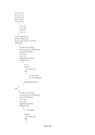
13. Write a program to perform reflection of two dimensional objects.
A) Y=0(X-axis) B) X=0(Y-axis) C) Y=X
Program:
# include <iostream.h>
# include <graphics.h>
# include <conio.h>
# include <math.h>
void show_screen( );
void apply_reflection_along_x_axis(const int,int []);
void apply_reflection_along_y_axis(const int,int []);
void apply_reflection_wrt_origin(const int,int []);
void multiply_matrices(const int[3],const int[3][3],int[3]);
void Polygon(const int,const int []);
void Line(const int,const int,const int,const int);
int main( )
{
int driver=VGA;
int mode=VGAHI;
initgraph(&driver,&mode,"..Bgi");
show_screen( );
setcolor(15);
Line(320,100,320,400);
Line(315,105,320,100);
Line(320,100,325,105);
Line(315,395,320,400);
Line(320,400,325,395);
Line(150,240,500,240);
Line(150,240,155,235);
Line(150,240,155,245);
Line(500,240,495,235);
Line(500,240,495,245);
settextstyle(2,0,4);
outtextxy(305,85,"y-axis");
outtextxy(305,402,"y'-axis");
outtextxy(505,233,"x-axis");
outtextxy(105,233,"x'-axis");
outtextxy(380,100,"Original Object");
outtextxy(380,385,"Reflection along x-axis");
outtextxy(135,100,"Reflection along y-axis");
outtextxy(135,385,"Reflection w.r.t origin");
int polygon_points[8]={ 350,200, 380,150, 470,200, 350,200 };
int x_polygon[8]={ 350,200, 380,150, 470,200, 350,200 };
int y_polygon[8]={ 350,200, 380,150, 470,200, 350,200 };
int origin_polygon[8]={ 350,200, 380,150, 470,200, 350,200 };
setcolor(15);
Polygon(4,polygon_points);
apply_reflection_along_x_axis(4,x_polygon);
setcolor(12);
Polygon(4,x_polygon);
apply_reflection_along_y_axis(4,y_polygon);](https://image.slidesharecdn.com/cgfile-140420070604-phpapp01/85/Computer-Graphics-Programes-47-320.jpg)
![Page | 48
setcolor(14);
Polygon(4,y_polygon);
apply_reflection_wrt_origin(4,origin_polygon);
setcolor(10);
Polygon(4,origin_polygon);
getch( );
return 0;
}
void apply_reflection_along_x_axis(const int n,int coordinates[])
{
for(int count=0;count<n;count++)
{
int matrix_a[3]={coordinates[(count*2)],coordinates[((count*2)+1)],1};
int matrix_b[3][3]={ {1,0,0} , {0,-1,0} ,{ 0,0,1} };
int matrix_c[3]={0};
multiply_matrices(matrix_a,matrix_b,matrix_c);
coordinates[(count*2)]=matrix_c[0];
coordinates[((count*2)+1)]=(480+matrix_c[1]);
}
}
void apply_reflection_along_y_axis(const int n,int coordinates[])
{
for(int count=0;count<n;count++)
{
int matrix_a[3]={coordinates[(count*2)],coordinates[((count*2)+1)],1};
int matrix_b[3][3]={ {-1,0,0} , {0,1,0} ,{ 0,0,1} };
int matrix_c[3]={0};
multiply_matrices(matrix_a,matrix_b,matrix_c);
coordinates[(count*2)]=(640+matrix_c[0]);
coordinates[((count*2)+1)]=matrix_c[1];
}
}
void apply_reflection_wrt_origin(const int n,int coordinates[])
{
for(int count=0;count<n;count++)
{
int matrix_a[3]={coordinates[(count*2)], coordinates[((count*2)+1)],1};
int matrix_b[3][3]={ {-1,0,0} , {0,-1,0} ,{ 0,0,1} };
int matrix_c[3]={0};
multiply_matrices(matrix_a,matrix_b,matrix_c);
coordinates[(count*2)]=(640+matrix_c[0]);
coordinates[((count*2)+1)]=(480+matrix_c[1]);
}
}
void multiply_matrices(const int matrix_1[3], const int matrix_2[3][3],int matrix_3[3])
{
for(int count_1=0;count_1<3;count_1++)
{
for(int count_2=0;count_2<3;count_2++)
matrix_3[count_1]+=
(matrix_1[count_2]*matrix_2[count_2][count_1]);](https://image.slidesharecdn.com/cgfile-140420070604-phpapp01/85/Computer-Graphics-Programes-48-320.jpg)
![Page | 49
}
}
void Polygon(const int n,const int coordinates[])
{
if(n>=2)
{
Line(coordinates[0],coordinates[1],coordinates[2],coordinates[3]);
for(int count=1;count<(n-1);count++)
Line(coordinates[(count*2)],coordinates[((count*2)+1)], coordinates[((count+1)*2)],
coordinates[(((count+1)*2)+1)]);
}
}
void Line(const int x_1,const int y_1,const int x_2,const int y_2)
{
int color=getcolor( );
int x1=x_1;
int y1=y_1;
int x2=x_2;
int y2=y_2;
if(x_1>x_2)
{
x1=x_2;
y1=y_2;
x2=x_1;
y2=y_1;
}
int dx=abs(x2-x1);
int dy=abs(y2-y1);
int inc_dec=((y2>=y1)?1:-1);
if(dx>dy)
{
int two_dy=(2*dy);
int two_dy_dx=(2*(dy-dx));
int p=((2*dy)-dx);
int x=x1;
int y=y1;
putpixel(x,y,color);
while(x<x2)
{
x++;
if(p<0)
p+=two_dy;
else
{
y+=inc_dec;
p+=two_dy_dx;
}
putpixel(x,y,color);
}
}](https://image.slidesharecdn.com/cgfile-140420070604-phpapp01/85/Computer-Graphics-Programes-49-320.jpg)
![Page | 51
Program:
# include <iostream.h>
# include <graphics.h>
# include <conio.h>
# include <math.h>
void show_screen( );
void apply_reflection_about_line_yex(const int,int []);
void apply_reflection_about_line_yemx(const int,int []);
void apply_reflection_along_x_axis(const int,int []);
void apply_reflection_along_y_axis(const int,int []);
void apply_rotation(const int,int [],float);
void multiply_matrices(const float[3],const float[3][3],float[3]);
void Polygon(const int,const int []);
void Line(const int,const int,const int,const int);
void Dashed_line(const int,const int,const int,const int,const int=0);
int main( )
{
int driver=VGA;
int mode=VGAHI;
initgraph(&driver,&mode,"..Bgi");
show_screen( );
setcolor(15);
Line(320,100,320,400);
Line(315,105,320,100);
Line(320,100,325,105);
Line(315,395,320,400);
Line(320,400,325,395);
Line(150,240,500,240);
Line(150,240,155,235);
Line(150,240,155,245);
Line(500,240,495,235);
Line(500,240,495,245);
Dashed_line(160,400,460,100,0);
Dashed_line(180,100,480,400,0);
settextstyle(2,0,4);
outtextxy(305,85,"y-axis");](https://image.slidesharecdn.com/cgfile-140420070604-phpapp01/85/Computer-Graphics-Programes-51-320.jpg)
![Page | 52
outtextxy(305,402,"y'-axis");
outtextxy(505,233,"x-axis");
outtextxy(105,233,"x'-axis");
outtextxy(350,100,"Reflection about the line y=x");
outtextxy(115,100,"Reflection about the line y=-x");
int x_polygon[8]={ 340,200, 420,120, 370,120, 340,200 };
int y_polygon[8]={ 300,200, 220,120, 270,120, 300,200 };
setcolor(15);
Polygon(4,x_polygon);
Polygon(4,y_polygon);
apply_reflection_about_line_yex(4,x_polygon);
apply_reflection_about_line_yemx(4,y_polygon);
setcolor(7);
Polygon(4,x_polygon);
Polygon(4,y_polygon);
getch( );
return 0;
}
void apply_reflection_about_line_yex(const int n,int coordinates[])
{
apply_rotation(n,coordinates,45);
apply_reflection_along_x_axis(n,coordinates);
apply_rotation(n,coordinates,-45);
}
void apply_reflection_about_line_yemx(const int n,int coordinates[])
{
apply_rotation(n,coordinates,45);
apply_reflection_along_y_axis(n,coordinates);
apply_rotation(n,coordinates,-45);
}
void apply_rotation(const int n,int coordinates[],float angle)
{
float xr=320;
float yr=240;
angle*=(M_PI/180);
for(int count_1=0;count_1<n;count_1++)
{
float matrix_a[3]={coordinates[(count_1*2)],coordinates[((count_1*2)+1)],1};
float temp_1=(((1-cos(angle))*xr)+(yr*sin(angle)));
float temp_2=(((1-cos(angle))*yr)-(xr*sin(angle)));
float matrix_b[3][3]={ { cos(angle),sin(angle),0 } , { -sin(angle),cos(angle),0 } ,
{ temp_1,temp_2,1 } };
float matrix_c[3]={0};
multiply_matrices(matrix_a,matrix_b,matrix_c);
coordinates[(count_1*2)]=(int)(matrix_c[0]+0.5);
coordinates[((count_1*2)+1)]=(int)(matrix_c[1]+0.5);
}
}
void apply_reflection_along_x_axis(const int n,int coordinates[])
{
for(int count=0;count<n;count++)](https://image.slidesharecdn.com/cgfile-140420070604-phpapp01/85/Computer-Graphics-Programes-52-320.jpg)
![Page | 53
{
float matrix_a[3]={coordinates[(count*2)],coordinates[((count*2)+1)],1};
float matrix_b[3][3]={ {1,0,0} , {0,-1,0} ,{ 0,0,1} };
float matrix_c[3]={0};
multiply_matrices(matrix_a,matrix_b,matrix_c);
coordinates[(count*2)]=matrix_c[0];
coordinates[((count*2)+1)]=(480+matrix_c[1]);
}
}
void apply_reflection_along_y_axis(const int n,int coordinates[])
{
for(int count=0;count<n;count++)
{
float matrix_a[3]={coordinates[(count*2)],coordinates[((count*2)+1)],1};
float matrix_b[3][3]={ {-1,0,0} , {0,1,0} ,{ 0,0,1} };
float matrix_c[3]={0};
multiply_matrices(matrix_a,matrix_b,matrix_c);
coordinates[(count*2)]=(640+matrix_c[0]);
coordinates[((count*2)+1)]=matrix_c[1];
}
}
void multiply_matrices(const float matrix_1[3], const float matrix_2[3][3],float matrix_3[3])
{
for(int count_1=0;count_1<3;count_1++)
{
for(int count_2=0;count_2<3;count_2++)
matrix_3[count_1]+=
(matrix_1[count_2]*matrix_2[count_2][count_1]);
}
}
void Polygon(const int n,const int coordinates[])
{
if(n>=2)
{
Line(coordinates[0],coordinates[1], coordinates[2],coordinates[3]);
for(int count=1;count<(n-1);count++)
Line(coordinates[(count*2)],coordinates[((count*2)+1)],coordinates[((count+1)*2)],
coordinates[(((count+1)*2)+1)]);
}
}
void Line(const int x_1,const int y_1,const int x_2,const int y_2)
{
int color=getcolor( );
int x1=x_1;
int y1=y_1;
int x2=x_2;
int y2=y_2;
if(x_1>x_2)
{
x1=x_2;
y1=y_2;](https://image.slidesharecdn.com/cgfile-140420070604-phpapp01/85/Computer-Graphics-Programes-53-320.jpg)
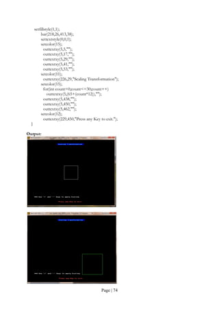
![Page | 58
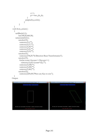
14. Write a program to perform shearing transformation in X direction.
Program:
# include <iostream.h>
# include <graphics.h>
# include <conio.h>
# include <math.h>
void show_screen( );
void apply_x_direction_shear(const int,int [],const float);
void multiply_matrices(const float[3],const float[3][3],float[3]);
void Polygon(const int,const int []);
void Line(const int,const int,const int,const int);
int main( )
{
int driver=VGA;
int mode=VGAHI;
initgraph(&driver,&mode,"..Bgi");
show_screen( );
int polygon_points[10]={ 270,340, 270,140, 370,140, 370,340, 270,340 };
setcolor(15);
Polygon(5,polygon_points);
setcolor(15);
settextstyle(0,0,1);
outtextxy(50,415,"*** Use Left and Right Arrow Keys to apply X-Direction Shear.");
int key_code_1=0;
int key_code_2=0;
char Key_1=NULL;
char Key_2=NULL;
do
{
Key_1=NULL;
Key_2=NULL;
key_code_1=0;
key_code_2=0;
Key_1=getch( );
key_code_1=int(Key_1);
if(key_code_1==0)
{
Key_2=getch( );
key_code_2=int(Key_2);
}
if(key_code_1==27)
break;
else if(key_code_1==0)
{
if(key_code_2==75)
{
setfillstyle(1,0);
bar(40,70,600,410);
apply_x_direction_shear(5,polygon_points,-0.1);](https://image.slidesharecdn.com/cgfile-140420070604-phpapp01/85/Computer-Graphics-Programes-58-320.jpg)
![Page | 59
setcolor(12);
Polygon(5,polygon_points);
}
else if(key_code_2==77)
{
setfillstyle(1,0);
bar(40,70,600,410);
apply_x_direction_shear(5,polygon_points,0.1);
setcolor(10);
Polygon(5,polygon_points);
}
}
}
while(1);
return 0;
}
void apply_x_direction_shear(const int n,int coordinates[],const float Sh_x)
{
for(int count=0;count<n;count++)
{
float matrix_a[3]={coordinates[(count*2)],coordinates[((count*2)+1)],1};
float matrix_b[3][3]={ {1,0,0} , {Sh_x,1,0} ,{ 0,0,1} };
float matrix_c[3]={0};
multiply_matrices(matrix_a,matrix_b,matrix_c);
coordinates[(count*2)]=(matrix_c[0]+0.5);
coordinates[((count*2)+1)]=(matrix_c[1]+0.5);
}
}
void multiply_matrices(const float matrix_1[3], const float matrix_2[3][3],float matrix_3[3])
{
for(int count_1=0;count_1<3;count_1++)
{
for(int count_2=0;count_2<3;count_2++)
matrix_3[count_1]+= (matrix_1[count_2]*matrix_2[count_2][count_1]);
}
}
void Polygon(const int n,const int coordinates[])
{
if(n>=2)
{
Line(coordinates[0],coordinates[1],coordinates[2],coordinates[3]);
for(int count=1;count<(n-1);count++)
Line(coordinates[(count*2)],coordinates[((count*2)+1)],
coordinates[((count+1)*2)],
coordinates[(((count+1)*2)+1)]);
}
}
void Line(const int x_1,const int y_1,const int x_2,const int y_2)
{
int color=getcolor( );](https://image.slidesharecdn.com/cgfile-140420070604-phpapp01/85/Computer-Graphics-Programes-59-320.jpg)
![Page | 62
15. Write a program to perform two successive translations.
Program:
# include <iostream.h>
# include <graphics.h>
# include <conio.h>
# include <math.h>
void show_screen( );
void apply_translation(const int,int [],const int,const int);
void multiply_matrices(const int[3],const int[3][3],int[3]);
void Polygon(const int,const int []);
void Line(const int,const int,const int,const int);
int main( )
{
int driver=VGA;
int mode=VGAHI;
initgraph(&driver,&mode,"..Bgi");
show_screen( );
int polygon_points[8]={ 270,290, 320,190, 370,290, 270,290 };
setcolor(15);
Polygon(4,polygon_points);
setcolor(15);
settextstyle(0,0,1);
outtextxy(50,415,"*** Use Arrow Keys to apply Translation.");
int key_code_1=0;
int key_code_2=0;
char Key_1=NULL;
char Key_2=NULL;
do
{
Key_1=NULL;
Key_2=NULL;
key_code_1=0;
key_code_2=0;
Key_1=getch( );
key_code_1=int(Key_1);
if(key_code_1==0)
{
Key_2=getch( );
key_code_2=int(Key_2);
}
if(key_code_1==27)
break;
else if(key_code_1==0)
{
if(key_code_2==72)
{
setfillstyle(1,0);
bar(40,70,600,410);
apply_translation(4,polygon_points,0,-25);](https://image.slidesharecdn.com/cgfile-140420070604-phpapp01/85/Computer-Graphics-Programes-62-320.jpg)
![Page | 63
setcolor(10);
Polygon(4,polygon_points);
}
else if(key_code_2==75)
{
setfillstyle(1,0);
bar(40,70,600,410);
apply_translation(4,polygon_points,-25,0);
setcolor(12);
Polygon(4,polygon_points);
}
else if(key_code_2==77)
{
setfillstyle(1,0);
bar(40,70,600,410);
apply_translation(4,polygon_points,25,0);
setcolor(14);
Polygon(4,polygon_points);
}
else if(key_code_2==80)
{
setfillstyle(1,0);
bar(40,70,600,410);
apply_translation(4,polygon_points,0,25);
setcolor(9);
Polygon(4,polygon_points);
}
}
}
while(1);
return 0;
}
void apply_translation(const int n,int coordinates[], const int Tx,const int Ty)
{
for(int count_1=0;count_1<n;count_1++)
{
int matrix_a[3]={coordinates[(count_1*2)],coordinates[((count_1*2)+1)],1};
int matrix_b[3][3]={ {1,0,0} , {0,1,0} ,{ Tx,Ty,1} };
int matrix_c[3]={0};
multiply_matrices(matrix_a,matrix_b,matrix_c);
coordinates[(count_1*2)]=matrix_c[0];
coordinates[((count_1*2)+1)]=matrix_c[1];
}
}
void multiply_matrices(const int matrix_1[3], const int matrix_2[3][3],int matrix_3[3])
{
for(int count_1=0;count_1<3;count_1++)
{
for(int count_2=0;count_2<3;count_2++)
matrix_3[count_1]+=
(matrix_1[count_2]*matrix_2[count_2][count_1]);](https://image.slidesharecdn.com/cgfile-140420070604-phpapp01/85/Computer-Graphics-Programes-63-320.jpg)
![Page | 64
}
}
void Polygon(const int n,const int coordinates[])
{
if(n>=2)
{
Line(coordinates[0],coordinates[1], coordinates[2],coordinates[3]);
for(int count=1;count<(n-1);count++)
Line(coordinates[(count*2)],coordinates[((count*2)+1)], coordinates[((count+1)*2)],
coordinates[(((count+1)*2)+1)]);
}
}
void Line(const int x_1,const int y_1,const int x_2,const int y_2)
{
int color=getcolor( );
int x1=x_1;
int y1=y_1;
int x2=x_2;
int y2=y_2;
if(x_1>x_2)
{
x1=x_2;
y1=y_2;
x2=x_1;
y2=y_1;
}
int dx=abs(x2-x1);
int dy=abs(y2-y1);
int inc_dec=((y2>=y1)?1:-1);
if(dx>dy)
{
int two_dy=(2*dy);
int two_dy_dx=(2*(dy-dx));
int p=((2*dy)-dx);
int x=x1;
int y=y1;
putpixel(x,y,color);
while(x<x2)
{
x++;
if(p<0)
p+=two_dy;
else
{
y+=inc_dec;
p+=two_dy_dx;
}
putpixel(x,y,color);
}
}](https://image.slidesharecdn.com/cgfile-140420070604-phpapp01/85/Computer-Graphics-Programes-64-320.jpg)
![Page | 67
16. Write a program to perform two successive Rotations.
Program:
# include <iostream.h>
# include <graphics.h>
# include <conio.h>
# include <math.h>
void show_screen( );
void apply_rotation(const int,int [],float);
void multiply_matrices(const float[3],const float[3][3],float[3]);
void Polygon(const int,const int []);
void Line(const int,const int,const int,const int);
int main( )
{
int driver=VGA;
int mode=VGAHI;
initgraph(&driver,&mode,"..Bgi");
show_screen( );
int polygon_points[8]={ 250,290, 320,190, 390,290, 250,290 };
setcolor(15);
Polygon(5,polygon_points);
setcolor(15);
settextstyle(0,0,1);
outtextxy(50,415,"*** Use '+' and '-' Keys to apply Rotation.");
int key_code=0;
char Key=NULL;
do
{
Key=NULL;
key_code=0;
Key=getch( );
key_code=int(Key);
if(key_code==0)
{
Key=getch( );
key_code=int(Key);
}
if(key_code==27)
break;
else if(key_code==43)
{
setfillstyle(1,0);
bar(40,70,600,410);
apply_rotation(4,polygon_points,5);
setcolor(10);
Polygon(4,polygon_points);
}
else if(key_code==45)
{
setfillstyle(1,0);](https://image.slidesharecdn.com/cgfile-140420070604-phpapp01/85/Computer-Graphics-Programes-67-320.jpg)
![Page | 68
bar(40,70,600,410);
apply_rotation(4,polygon_points,-5);
setcolor(12);
Polygon(4,polygon_points);
}
}
while(1);
return 0;
}
void apply_rotation(const int n,int coordinates[],float angle)
{
angle*=(M_PI/180);
for(int count_1=0;count_1<n;count_1++)
{
float matrix_a[3]={coordinates[(count_1*2)],coordinates[((count_1*2)+1)],1}; float
matrix_b[3][3]={ { cos(angle),sin(angle),0 } ,{ -sin(angle),cos(angle),0 } ,{ 0,0,1 } };
float matrix_c[3]={0};
multiply_matrices(matrix_a,matrix_b,matrix_c);
coordinates[(count_1*2)]=(int)(matrix_c[0]+0.5);
coordinates[((count_1*2)+1)]=(int)(matrix_c[1]+0.5);
}
}
void multiply_matrices(const float matrix_1[3],const float matrix_2[3][3],float matrix_3[3])
{
for(int count_1=0;count_1<3;count_1++)
{
for(int count_2=0;count_2<3;count_2++)
matrix_3[count_1]+=
(matrix_1[count_2]*matrix_2[count_2][count_1]);
}
}
void Polygon(const int n,const int coordinates[])
{
if(n>=2)
{
Line(coordinates[0],coordinates[1], coordinates[2],coordinates[3]);
for(int count=1;count<(n-1);count++)
Line(coordinates[(count*2)],coordinates[((count*2)+1)], coordinates[((count+1)*2)],
coordinates[(((count+1)*2)+1)]);
}
}
void Line(const int x_1,const int y_1,const int x_2,const int y_2)
{
int color=getcolor( );
int x1=x_1;
int y1=y_1;
int x2=x_2;
int y2=y_2;
if(x_1>x_2)
{
x1=x_2;](https://image.slidesharecdn.com/cgfile-140420070604-phpapp01/85/Computer-Graphics-Programes-68-320.jpg)
![Page | 71
17. Write a program to perform two successive scaling.
Program:
# include <iostream.h>
# include <graphics.h>
# include <conio.h>
# include <math.h>
void show_screen( );
void apply_scaling(const int,int [],const float,const float);
void multiply_matrices(const float[3],const float[3][3],float[3]);
void Polygon(const int,const int []);
void Line(const int,const int,const int,const int);
int main( )
{
int driver=VGA;
int mode=VGAHI;
initgraph(&driver,&mode,"..Bgi");
show_screen( );
int polygon_points[10]={ 270,290, 270,190, 370,190, 370,290, 270,290 };
setcolor(15);
Polygon(5,polygon_points);
setcolor(15);
settextstyle(0,0,1);
outtextxy(50,415,"*** Use '+' and '-' Keys to apply Scaling.");
int key_code=0;
char Key=NULL;
do
{
Key=NULL;
key_code=0;
Key=getch( );
key_code=int(Key);
if(key_code==0)
{
Key=getch( );
key_code=int(Key);
}
if(key_code==27)
break;
else if(key_code==43)
{
setfillstyle(1,0);
bar(40,70,600,410);
apply_scaling(5,polygon_points,1.1,1.1);
setcolor(10);
Polygon(5,polygon_points);
}
else if(key_code==45)
{
setfillstyle(1,0);
bar(40,70,600,410);](https://image.slidesharecdn.com/cgfile-140420070604-phpapp01/85/Computer-Graphics-Programes-71-320.jpg)
![Page | 72
apply_scaling(5,polygon_points,0.9,0.9);
setcolor(12);
Polygon(5,polygon_points);
}
}
while(1);
return 0;
}
void apply_scaling(const int n,int coordinates[],const float Sx,const float Sy)
{
for(int count_1=0;count_1<n;count_1++)
{
float matrix_a[3]={coordinates[(count_1*2)], coordinates[((count_1*2)+1)],1};
float matrix_b[3][3]={ {Sx,0,0} , {0,Sy,0} ,{ 0,0,1} };
float matrix_c[3]={0};
multiply_matrices(matrix_a,matrix_b,matrix_c);
coordinates[(count_1*2)]=(int)(matrix_c[0]+0.5);
coordinates[((count_1*2)+1)]=(int)(matrix_c[1]+0.5);
}
}
void multiply_matrices(const float matrix_1[3],const float matrix_2[3][3],float matrix_3[3])
{
for(int count_1=0;count_1<3;count_1++)
{
for(int count_2=0;count_2<3;count_2++)
matrix_3[count_1]+=
(matrix_1[count_2]*matrix_2[count_2][count_1]);
}
}
void Polygon(const int n,const int coordinates[])
{
if(n>=2)
{
Line(coordinates[0],coordinates[1], coordinates[2],coordinates[3]);
for(int count=1;count<(n-1);count++)
Line(coordinates[(count*2)],coordinates[((count*2)+1)],coordinates[((count+1)*2)],
coordinates[(((count+1)*2)+1)]);
}
}
void Line(const int x_1,const int y_1,const int x_2,const int y_2)
{
int color=getcolor( );
int x1=x_1;
int y1=y_1;
int x2=x_2;
int y2=y_2;
if(x_1>x_2)
{
x1=x_2;
y1=y_2;](https://image.slidesharecdn.com/cgfile-140420070604-phpapp01/85/Computer-Graphics-Programes-72-320.jpg)

The document discusses various graphics concepts used in C programming including: 1. Color constants, fill patterns, graphics drivers, errors, and modes that are used in graphics functions. 2. The functions closegraph, detectgraph, getbkcolor, getcolor, getmaxx, getmaxy, getpixel, getx, gety, grapherrormsg, graphresult, initgraph, outtext, outtexttxy, putpixel, setbkcolor, setcolor, and setfillpattern and their purposes. 3. initgraph initializes the graphics system by loading a driver and putting the system into graphics mode, while closegraph deallocates memory and restores the original screen mode.