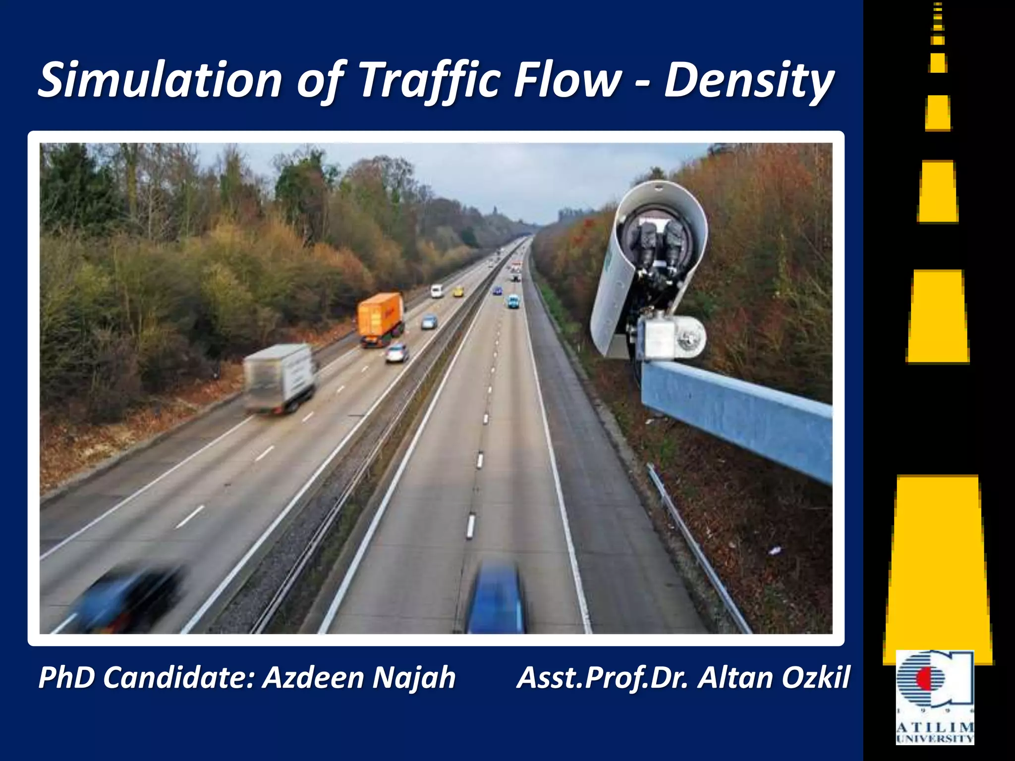
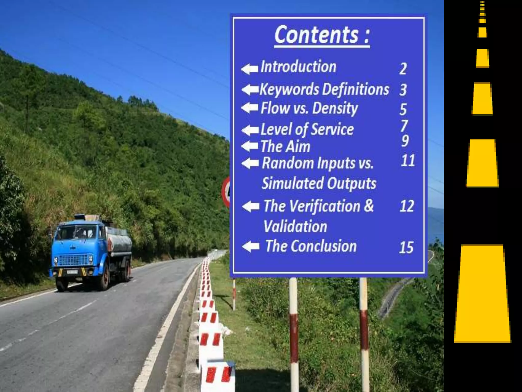
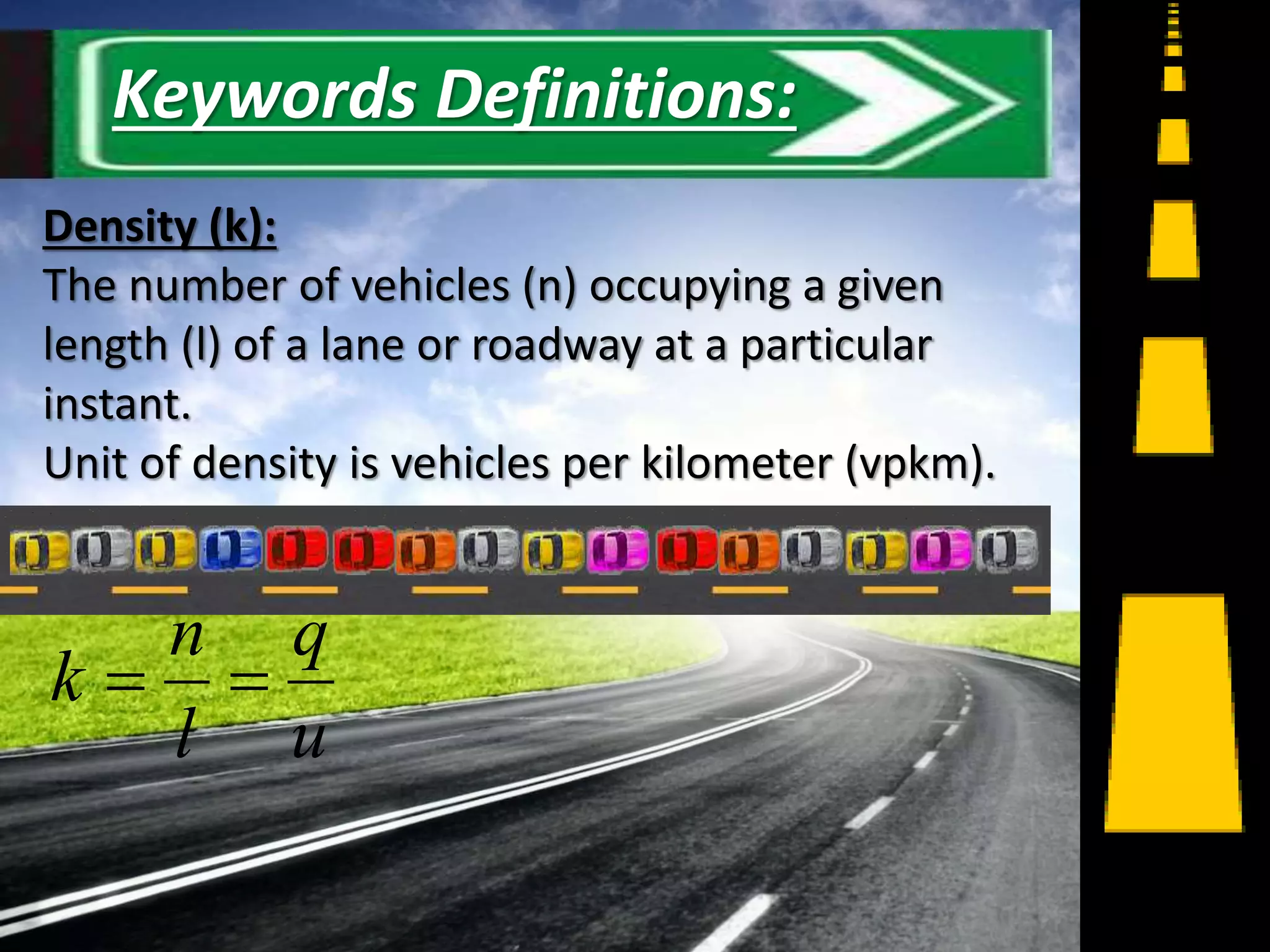
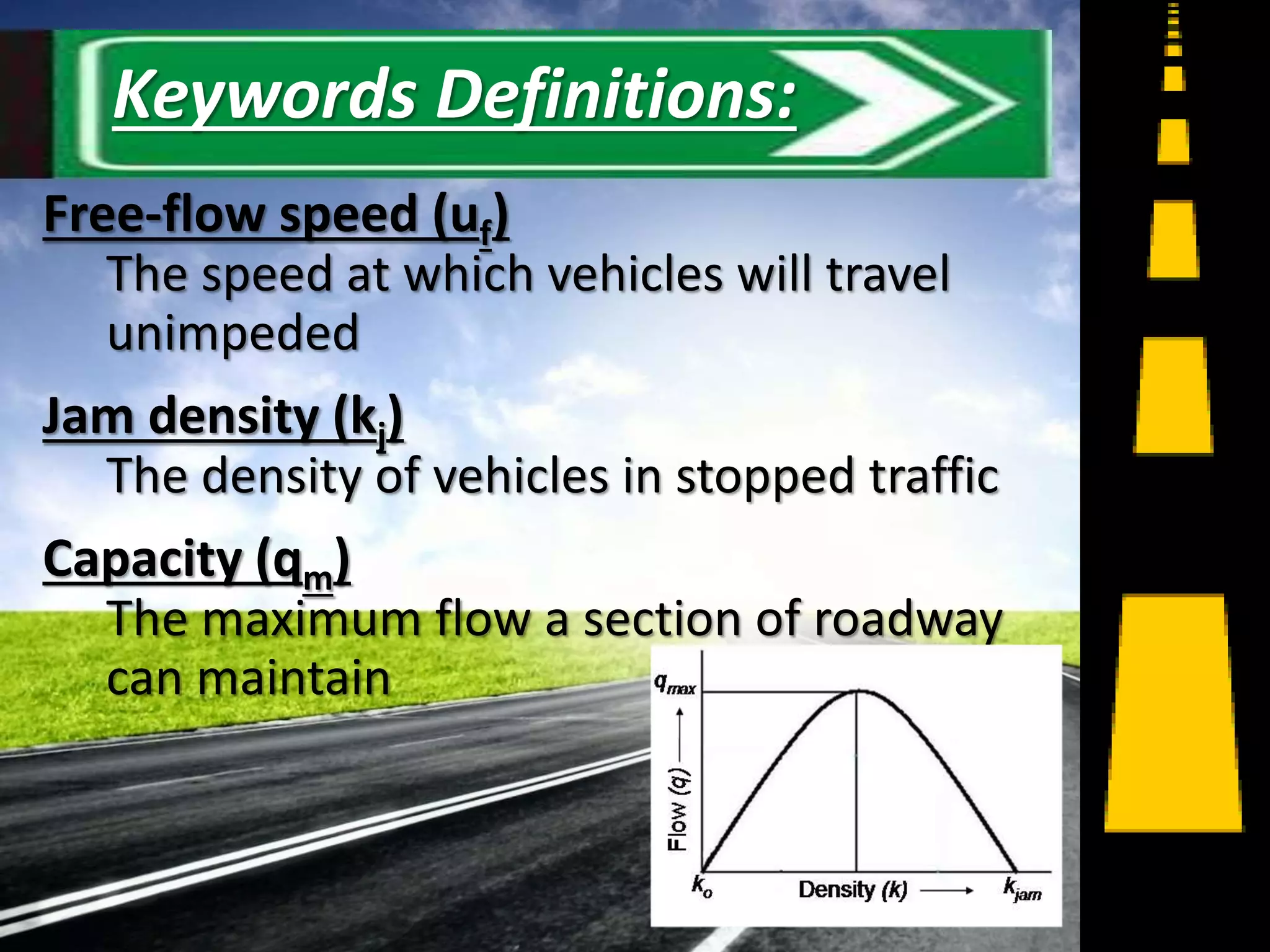
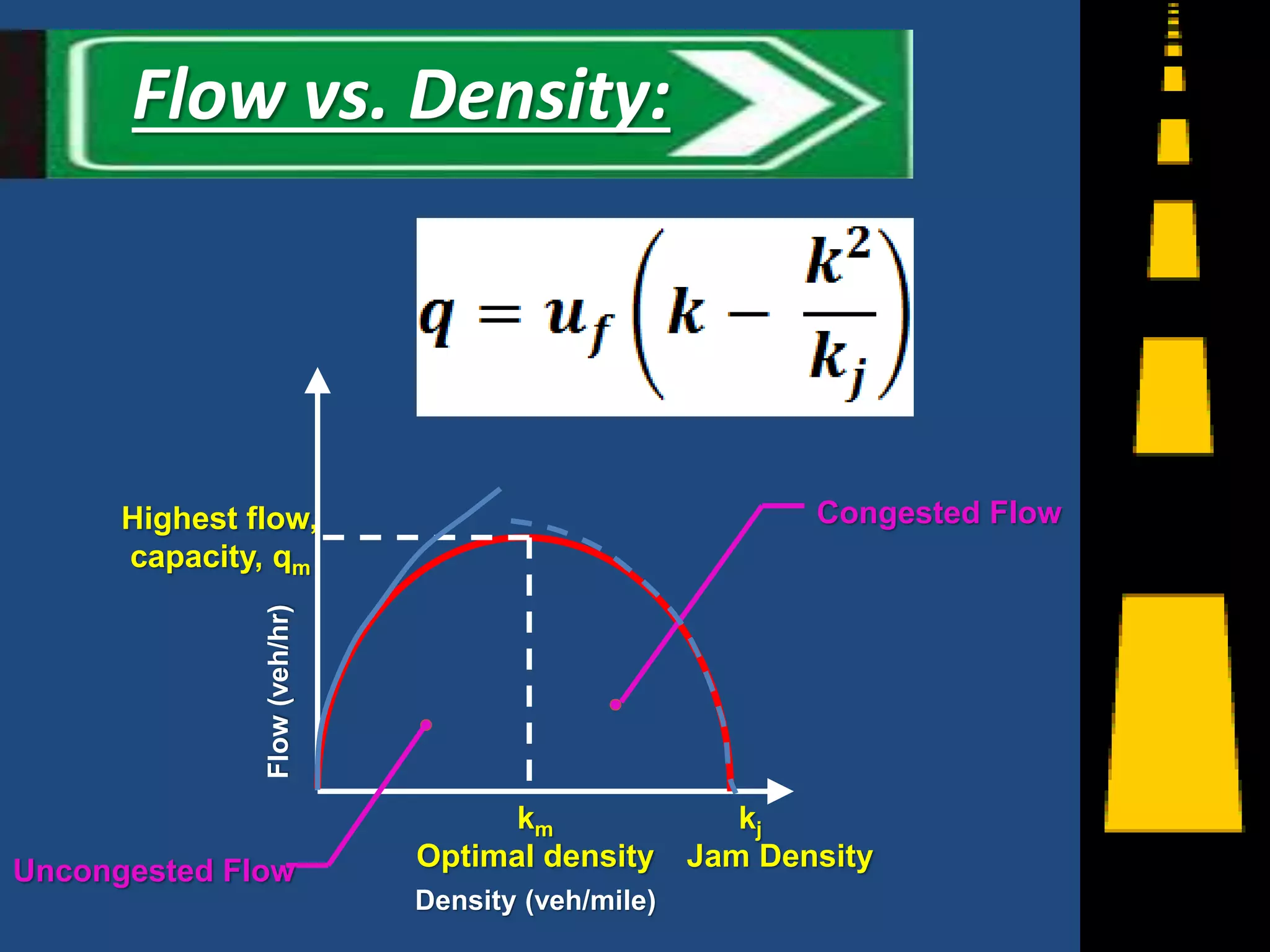
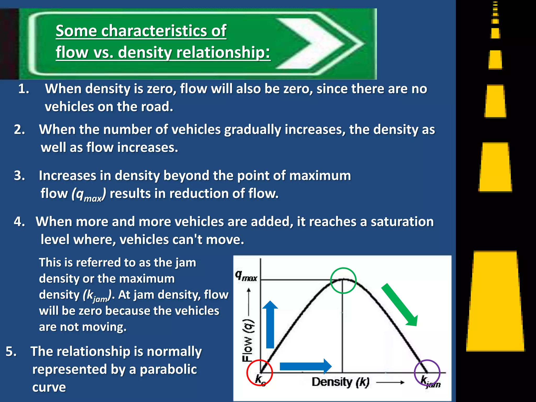
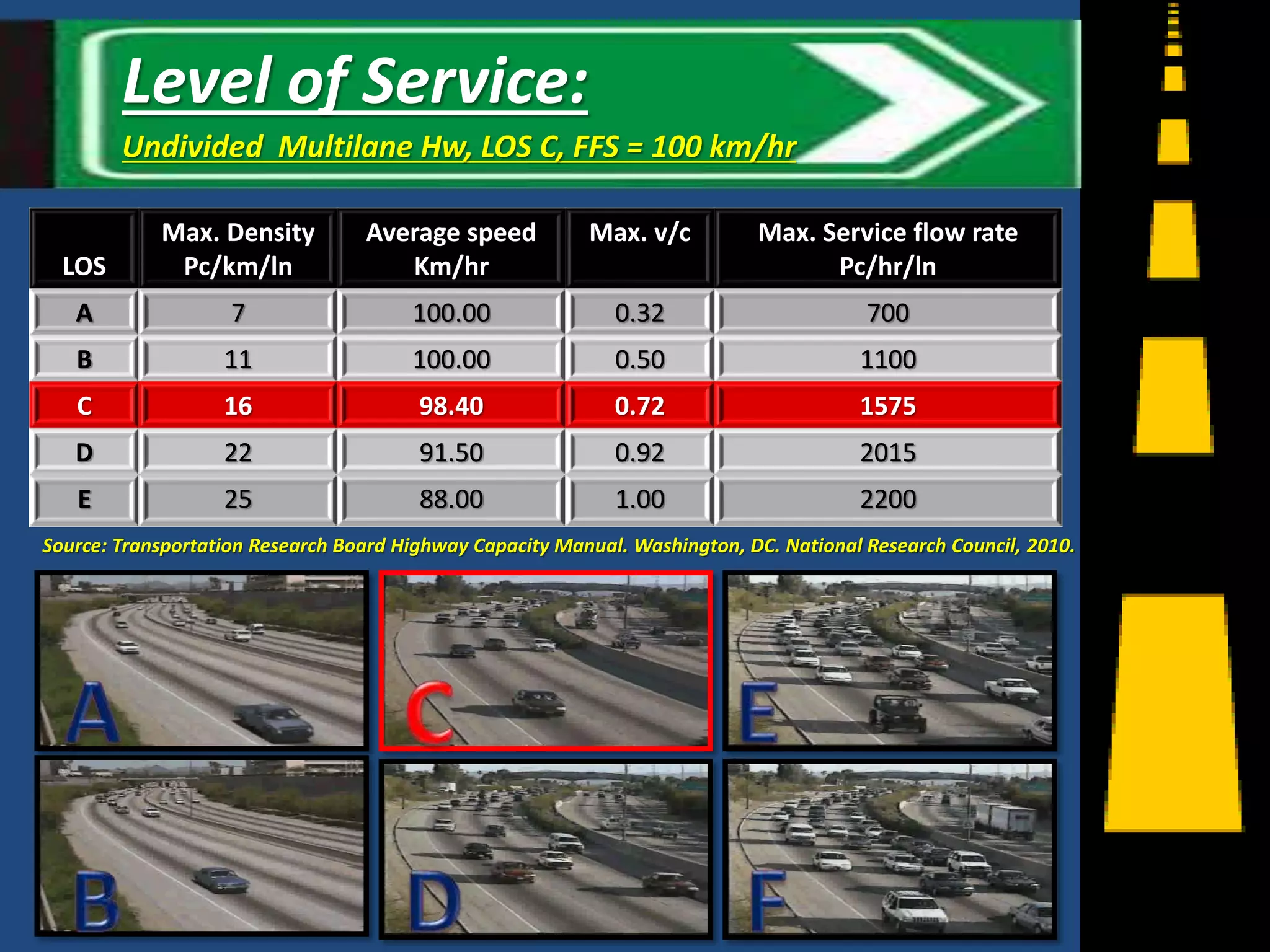
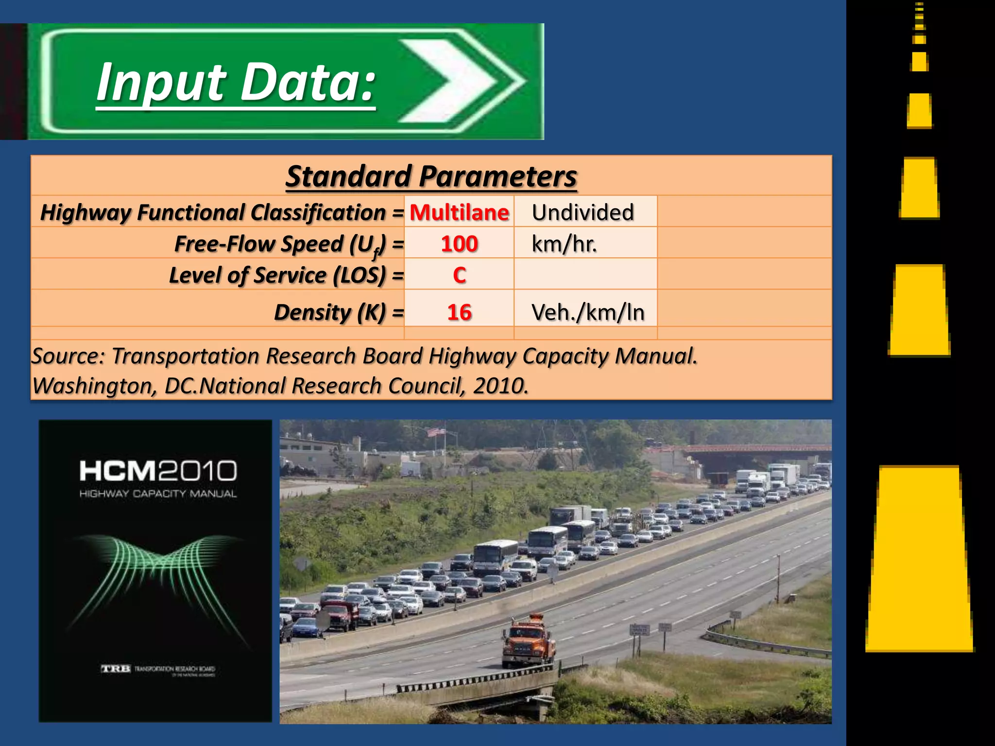
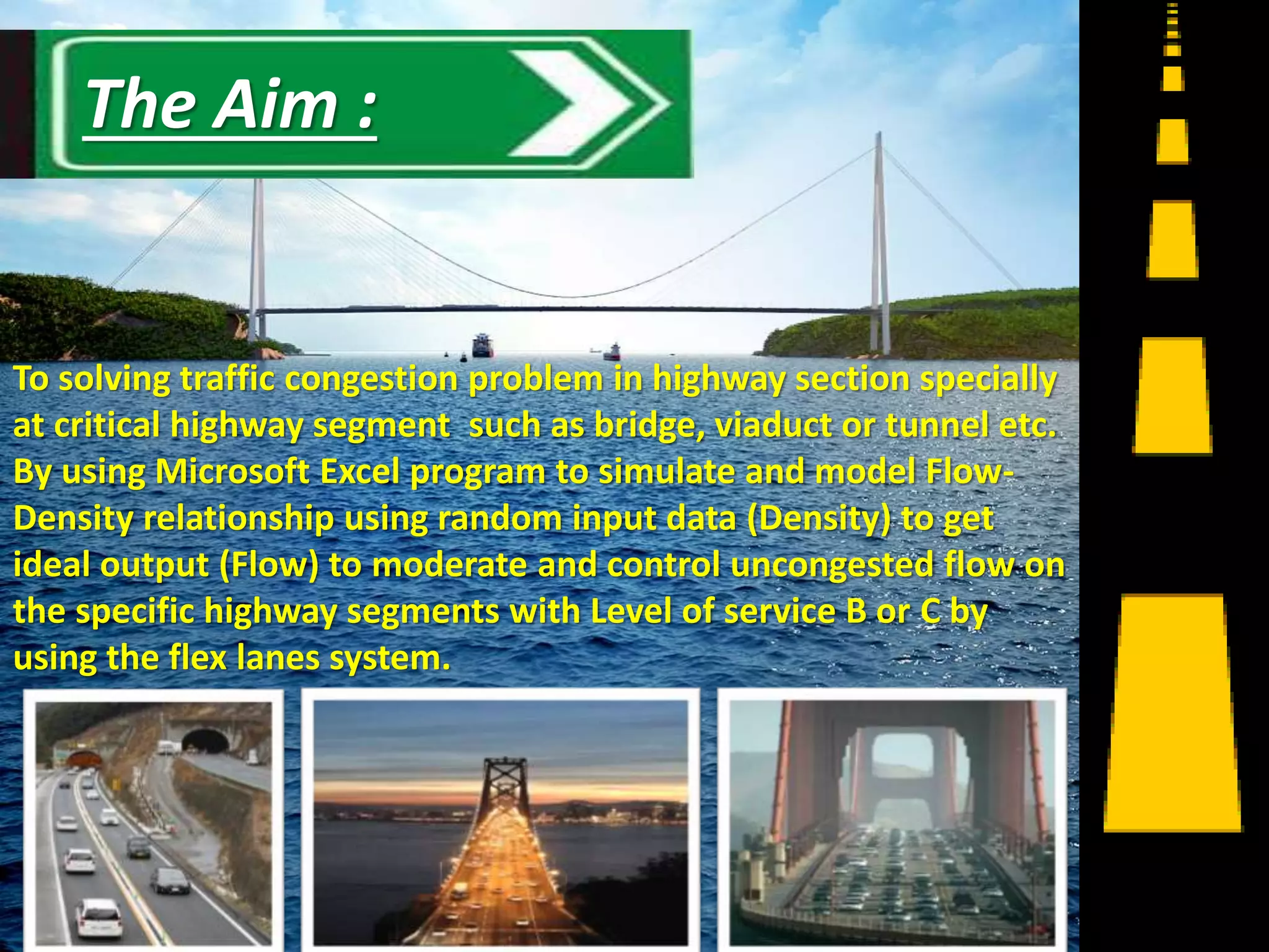
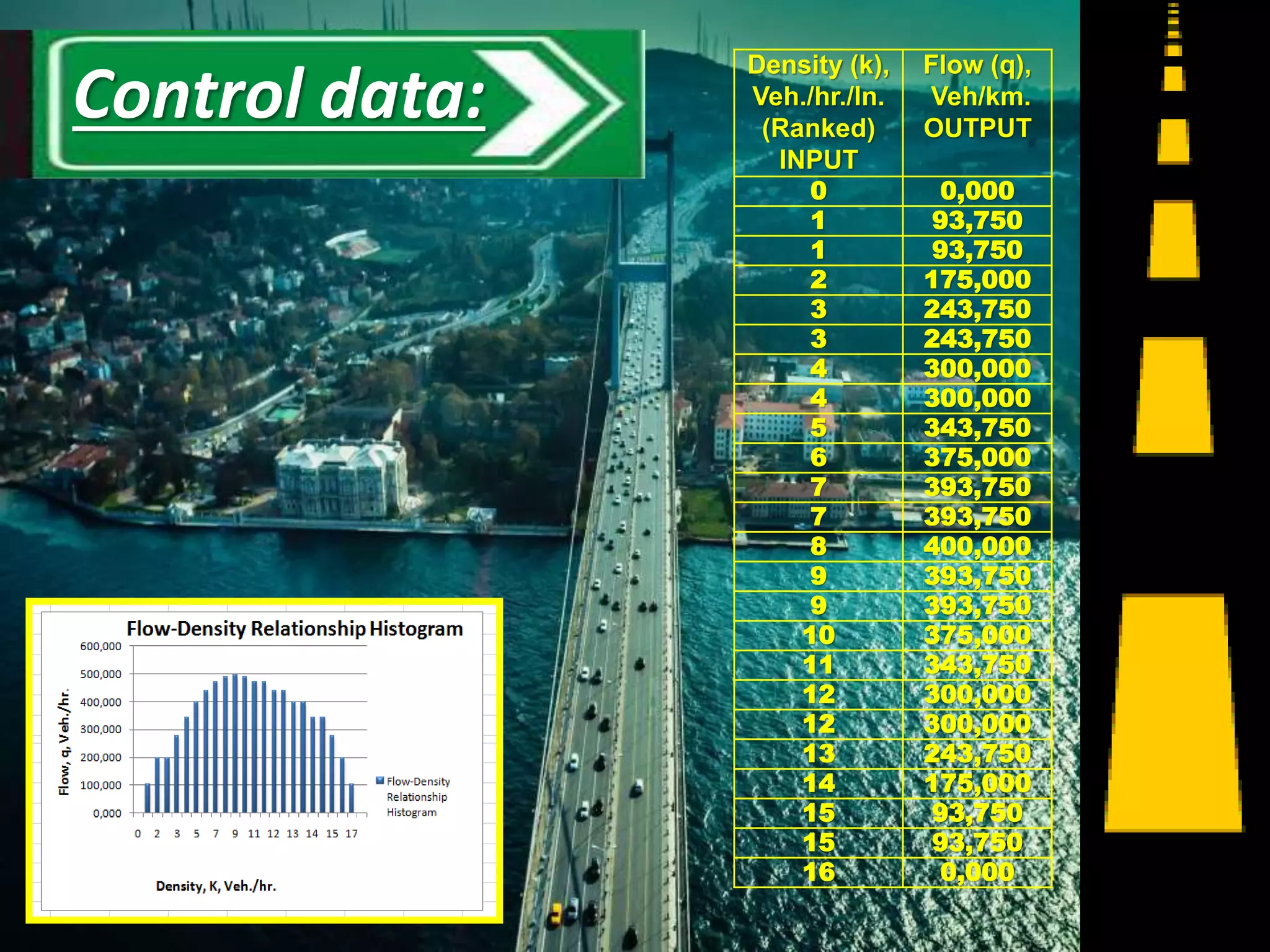
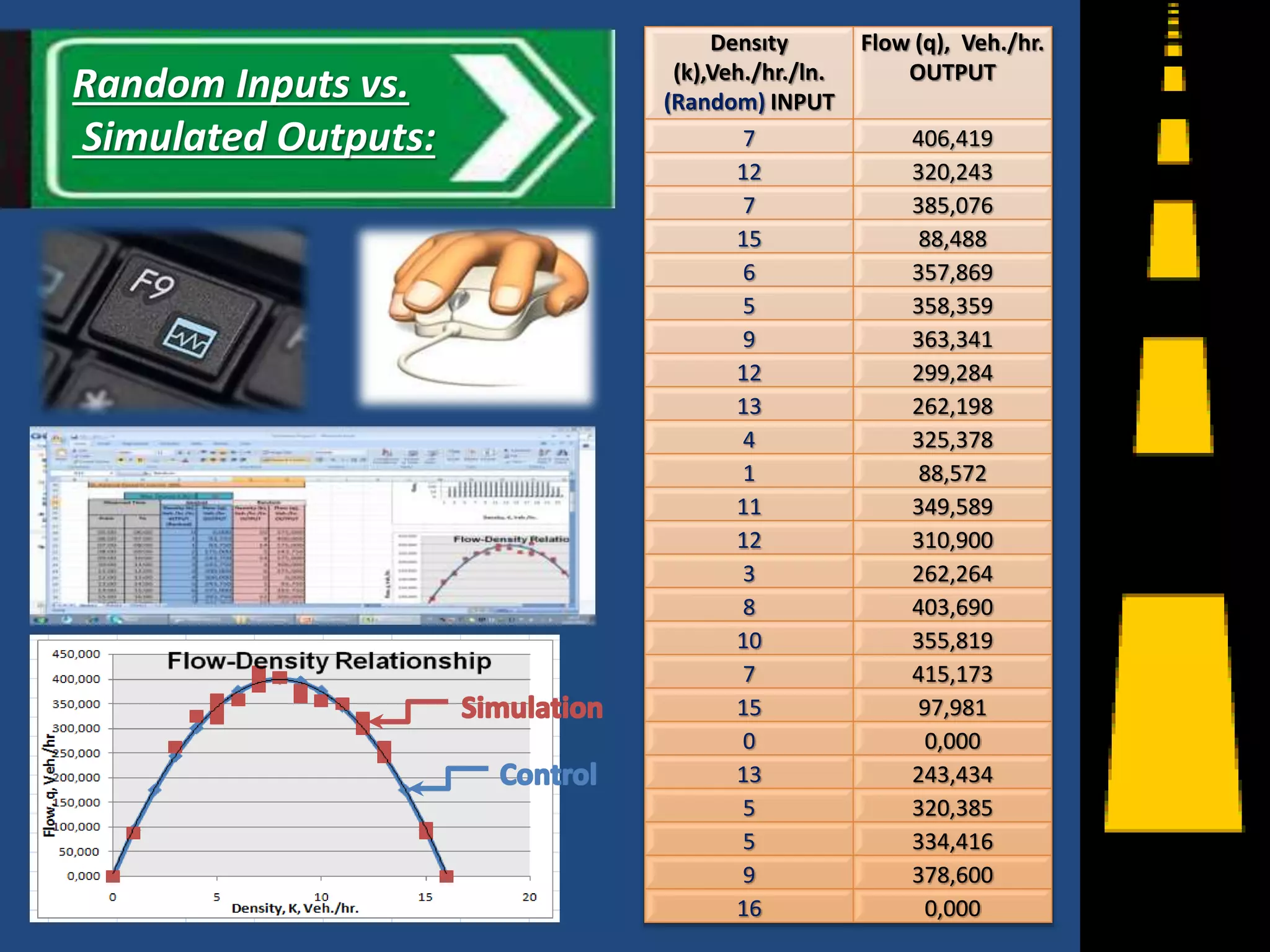
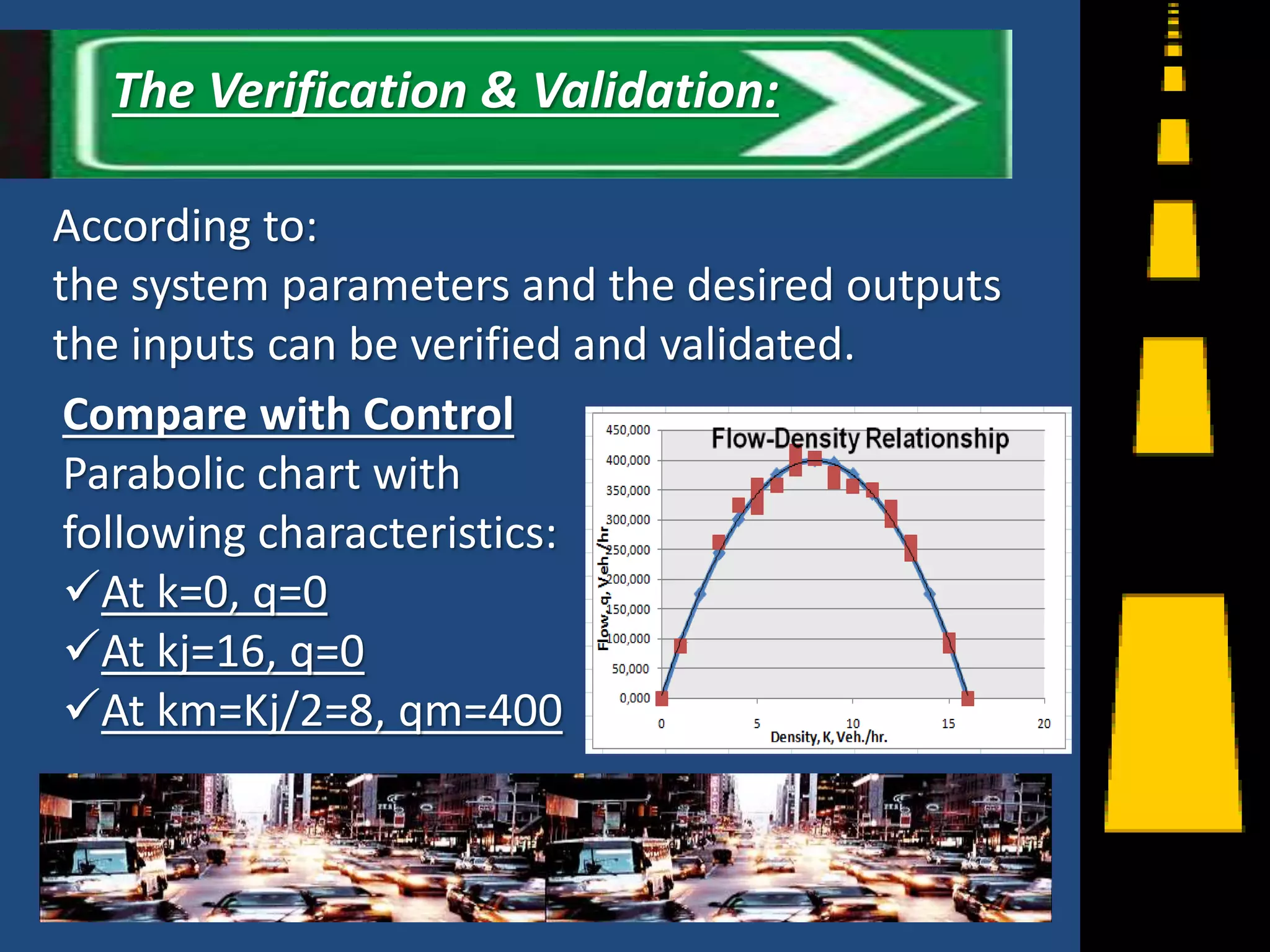
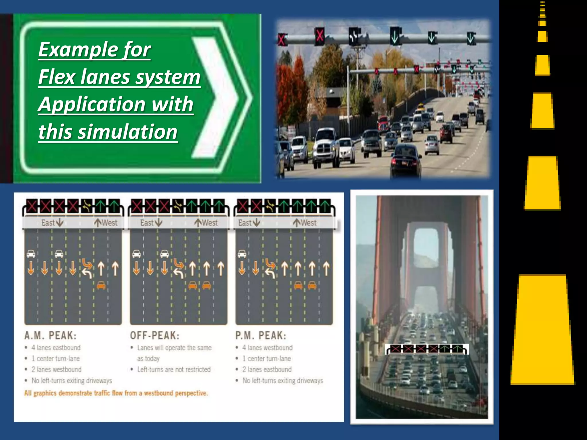
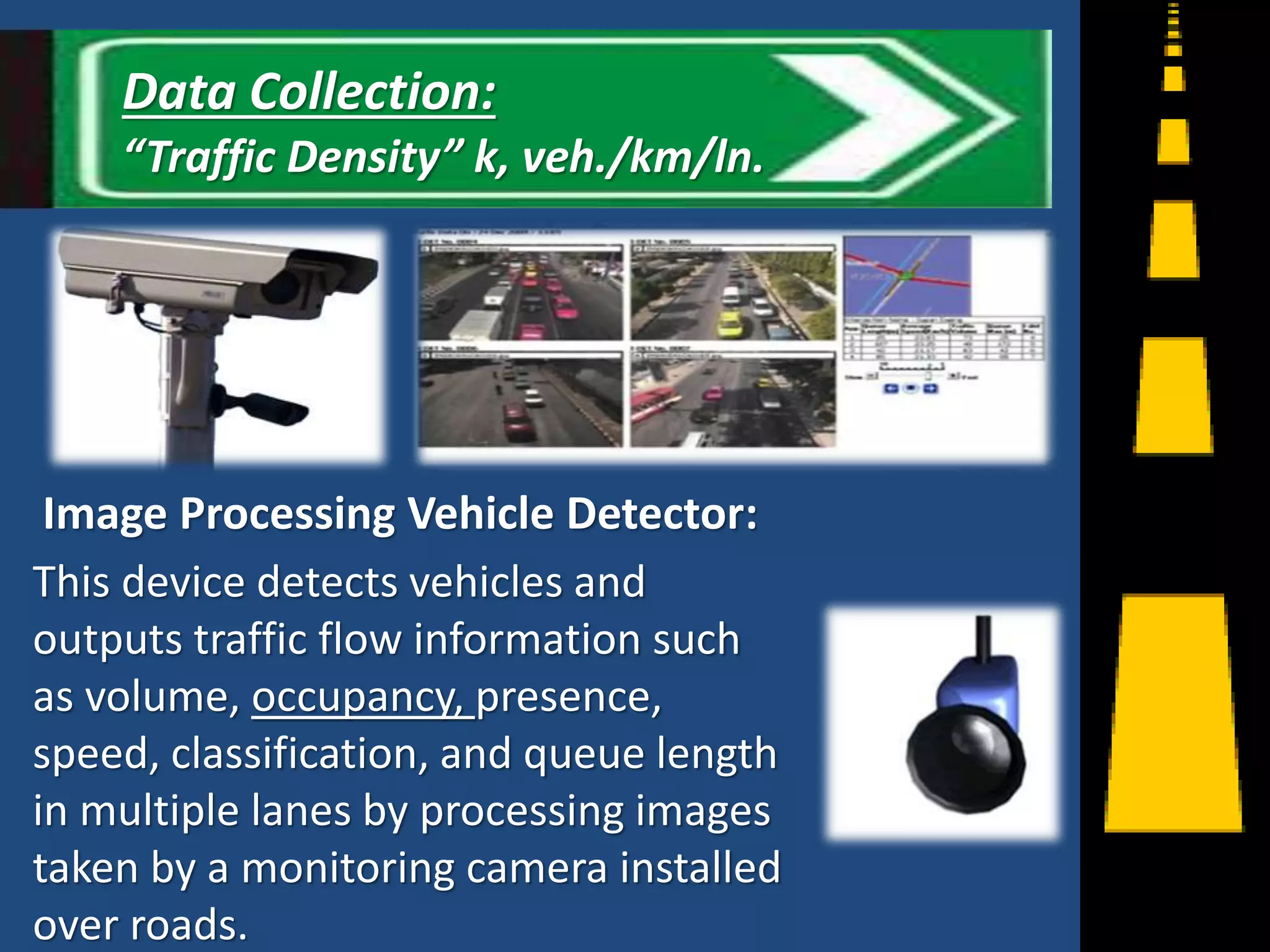
The document discusses the simulation of traffic flow, focusing on the relationship between vehicle density and flow characteristics. Key concepts include various definitions of density, flow, jam density, and their impact on traffic congestion, particularly in critical segments like bridges and tunnels. The study aims to model and control traffic flow using input data to optimize road capacity and improve level of service under different conditions.

1. Simulation of Traffic Flow - Density
PhD Candidate: Azdeen Najah Asst.Prof.Dr. Altan Ozkil
1

2. 2

3. 3
Introduction:

4. Density (k):
The number of vehicles (n) occupying a given
length (l) of a lane or roadway at a particular
instant.
Unit of density is vehicles per kilometer (vpkm).
u
q
l
n
k 
4
Keywords Definitions:

5. Free-flow speed (uf)
The speed at which vehicles will travel
unimpeded
Jam density (kj)
The density of vehicles in stopped traffic
Capacity (qm)
The maximum flow a section of roadway
can maintain
5
Keywords Definitions:

6. Density (veh/mile)
Flow(veh/hr)
kj
Jam Density
Highest flow,
capacity, qm
km
Optimal densityUncongested Flow
Congested Flow
6
Flow vs. Density:

7. 1. When density is zero, flow will also be zero, since there are no
vehicles on the road.
2. When the number of vehicles gradually increases, the density as
well as flow increases.
3. Increases in density beyond the point of maximum
flow (qmax) results in reduction of flow.
4. When more and more vehicles are added, it reaches a saturation
level where, vehicles can't move.
5. The relationship is normally
represented by a parabolic
curve 7
Some characteristics of
flow vs. density relationship:
This is referred to as the jam
density or the maximum
density (kjam). At jam density, flow
will be zero because the vehicles
are not moving.

8. LOS
Max. Density
Pc/km/ln
Average speed
Km/hr
Max. v/c Max. Service flow rate
Pc/hr/ln
A 7 100.00 0.32 700
B 11 100.00 0.50 1100
C 16 98.40 0.72 1575
D 22 91.50 0.92 2015
E 25 88.00 1.00 2200
Source: Transportation Research Board Highway Capacity Manual. Washington, DC. National Research Council, 2010.
8
Level of Service:
Undivided Multilane Hw, LOS C, FFS = 100 km/hr

9. Standard Parameters
Highway Functional Classification = Multilane Undivided
Free-Flow Speed (Uf) = 100 km/hr.
Level of Service (LOS) = C
Density (K) = 16 Veh./km/ln
Source: Transportation Research Board Highway Capacity Manual.
Washington, DC.National Research Council, 2010.
9
Input Data:

10. To solving traffic congestion problem in highway section specially
at critical highway segment such as bridge, viaduct or tunnel etc.
By using Microsoft Excel program to simulate and model Flow-
Density relationship using random input data (Density) to get
ideal output (Flow) to moderate and control uncongested flow on
the specific highway segments with Level of service B or C by
using the flex lanes system.
10
The Aim :

11. Density (k),
Veh./hr./ln.
(Ranked)
INPUT
Flow (q),
Veh/km.
OUTPUT
0 0,000
1 93,750
1 93,750
2 175,000
3 243,750
3 243,750
4 300,000
4 300,000
5 343,750
6 375,000
7 393,750
7 393,750
8 400,000
9 393,750
9 393,750
10 375,000
11 343,750
12 300,000
12 300,000
13 243,750
14 175,000
15 93,750
15 93,750
16 0,000
11
Control data:

12. Densıty
(k),Veh./hr./ln.
(Random) INPUT
Flow (q), Veh./hr.
OUTPUT
7 406,419
12 320,243
7 385,076
15 88,488
6 357,869
5 358,359
9 363,341
12 299,284
13 262,198
4 325,378
1 88,572
11 349,589
12 310,900
3 262,264
8 403,690
10 355,819
7 415,173
15 97,981
0 0,000
13 243,434
5 320,385
5 334,416
9 378,600
16 0,000 12
Random Inputs vs.
Simulated Outputs:

13. According to:
the system parameters and the desired outputs
the inputs can be verified and validated.
Compare with Control
Parabolic chart with
following characteristics:
At k=0, q=0
At kj=16, q=0
At km=Kj/2=8, qm=400
13
The Verification & Validation:

14. 14
Example for
Flex lanes system
Application with
this simulation

15. Image Processing Vehicle Detector:
This device detects vehicles and
outputs traffic flow information such
as volume, occupancy, presence,
speed, classification, and queue length
in multiple lanes by processing images
taken by a monitoring camera installed
over roads.
15
Data Collection:
“Traffic Density” k, veh./km/ln.

16. For Determine the traffic flow and capacity for
any road segment we should know its functional
classification, LOS, FFS and Number & width of
lanes.
By using Simulation and modelling we can solve
the traffic congestion problems by moderate and
control the critical highway segments such as
viaducts, bridges and tunnels.
16
The Conclusion:

17. Transportation Research Board
Highway Capacity Manual.
Washington, DC. National Research
Council, 2010.
Principles of Highway Engineering
and Traffic Analysis. 3dh. Edition.
17
The References:

18. 18