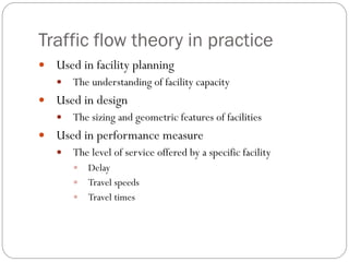
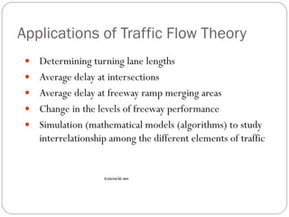
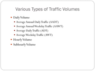
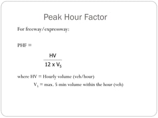
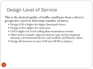
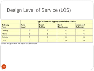
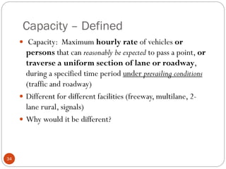
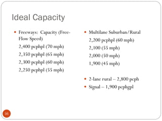
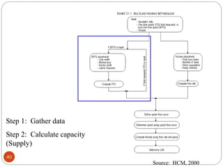
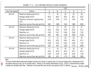
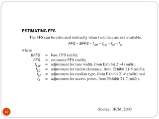
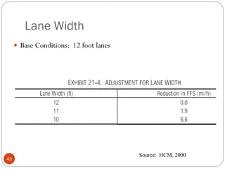
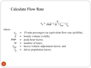
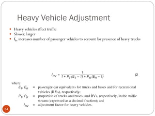
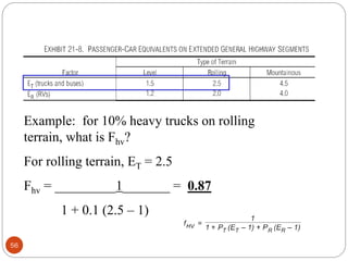
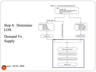
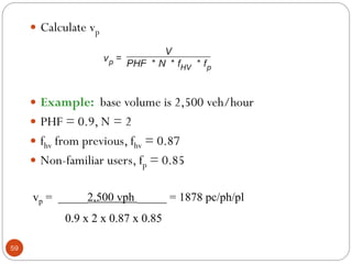
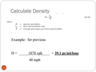
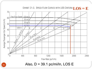
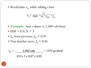
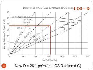
This document discusses various concepts in transportation engineering related to traffic flow theory and capacity analysis. It provides definitions and examples of key terms including: - Average daily traffic and peak hour factors which are used to determine directional design hourly volume - Applications of traffic flow theory such as determining turning lane lengths and delays - Level of service which is a qualitative measure of operational conditions within a traffic stream - Capacity, which is the maximum hourly rate of vehicles that can reasonably pass a point under prevailing conditions - Methods for calculating capacity and adjusting for factors like lane width, lateral clearance, and heavy vehicles using equations from the Highway Capacity Manual.

1. Transportation Engineering
Lina Shbeeb
Capacity Analysis

2. Traffic flow theory in practice
 Used in facility planning
 The understanding of facility capacity
 Used in design
 The sizing and geometric features of facilities
 Used in performance measure
 The level of service offered by a specific facility
 Delay
 Travel speeds
 Travel times

3. Applications of Traffic Flow Theory
 Determining turning lane lengths
 Average delay at intersections
 Average delay at freeway ramp merging areas
 Change in the levels of freeway performance
 Simulation (mathematical models (algorithms) to study
interrelationship among the different elements of traffic
itcdemo3d.ram

4. Various Types of Traffic Volumes
 DailyVolume
 AverageAnnual DailyTraffic (AADT)
 AverageAnnualWeekdayTraffic (AAWT)
 Average DailyTraffic (ADT)
 AverageWeekdayTraffic (AWT)
 HourlyVolume
 SubhourlyVolume

5. AADT and AAWT
 AverageAnnual DailyTraffic (AADT)
 Average 24-hour traffic volume at a location over a full 365-day
year, which is the total number of vehicles passing the location
divided by 365
 AverageAnnualWeekdayTraffic (AAWT)
 Average 24-hour traffic volume on weekdays over a full year,
which is the total weekday traffic volume divided by 260

6. ADT and AWT
 Average DailyTraffic (ADT)
 Average 24-hour traffic at a location for any period less than a
year (e.g. six months, a season, a month, a week or even two
days)
 AverageWeekdayTraffic (AWT)
 Average 24-hour traffic volume on weekdays for any period less
than a year

7. DDHV/PHV
 Directional Design Hourly volume (DDHV) ~ Peak
HourlyVolume
DDHV (veh/hour) =AADT x K x D
where AADT = Average Annual DailyTraffic (veh/day)
K = Proportion of daily traffic occurring in
peak hour (decimal)
D = Proportion of peak hour traffic traveling
in the peak direction (decimal)
Contd…

8. DDHV/PHV
 For design purposes, K factor is generally chosen as 30 HV and D
factor as the percentage of traffic in predominant direction during
the design hour
 General ranges for K and D factors
Facility Type K Factor D Factor
Rural 0.15 – 0.25 0.65 – 0.80
Suburban 0.12 – 0.15 0.55 – 0.65
Urban 0.07 – 0.12 0.50 – 0.60

9. Sub-Hourly Volume
 Sub-hourlyVolume ~ 15-minVolume
Suppose, the peak 15-min volume observed = 750 veh
So, the HourlyVolume =
15-min volume x 4
= 750 x 4
= 3000 veh/hour

10. Peak Hour Factor
 Relationship between hourly volume and maximum
rate of flow within the hour
For intersection:
PHF = =
where HV = Hourly volume (veh/hour)
V15 = max. 15-min volume within the hour (veh)
Hourly Volume
Max. Rate of Flow
HV
4 x V15

11. Example of PHF Calculation
 Data collected are as follows:
Time Interval Volume (veh)
4:00-4:15 pm 950
4:15-4:30 pm 1100
4:30-4:45 pm 1200
4:45-5:00 pm 1050
Hourly Volume 4300

12. Example of PHF Calculation
We find from the table,
HV = 4300 veh/hour
V15 = 1200 veh
Therefore,
PHF = = = 0.90
HV
4 x V15
4300
4 x 1200

13. Peak Hour Factor
For freeway/expressway:
PHF =
where HV = Hourly volume (veh/hour)
V5 = max. 5-min volume within the hour (veh)
HV
12 x V5

14. Traffic Volume
 Number of vehicles passing a given point or a section of a
roadway during a specified time
 Data collected by
 Manual counting
 Electro-mechanical devices

15. Relationship of Highest Hourly Volume and
ADT on Rural Arterials

16. Travel Time and Delay Surveys
 Want to determine travel time between two points or causes of
delay along a route
 Used for
Performance monitoring
Before and after evaluation of traffic management
schemes or new infrastructure

17. Stream measurements: the moving
observer method
 Moving Observer
 stopwatch, pen and paper
 laptop PC
 instrumented vehicle
=> Chase car versus floating car techniques
 Stationary Observer
 number plate survey
 Field staff or optical character recognition from video
 Vehicle electronic tags
 Mobile phone

18. Travel Time
By travelling several times in a car fromA to B, a
person notes down the time taken in each run and
then comes up with a statistical average ofTravel
Time.
A
B

19. Delay
Delay =Actual travel time - Expected travel time
 Stopped time delay
 Travel time delay

20. Calculation of Delay
 Travel time delay
 Actual travel time data collected by traveling in a car through
the stretch of the road under study.
 Expected travel time calculated from the distance and average
speed.
 Travel time delay calculated from the difference between actual
travel time and expected travel time.
 Stopped time data for the vehicular speed of 0 to 5 mph.

21. Introduction
 Shock wave - a rapid change in traffic conditions (speed,
density, and flow)
 A moving boundary between two different traffic states
 Forward, backward, and stationary shock waves

22. Travel Time
By travelling several times in a car fromA to B, a
person notes down the time taken in each run and
then comes up with a statistical average ofTravel
Time.
A
B

23. Delay
Delay =Actual travel time - Expected travel time
 Stopped time delay
 Travel time delay

24. Calculation of Delay
 Travel time delay
 Actual travel time data collected by traveling in a car through
the stretch of the road under study.
 Expected travel time calculated from the distance and average
speed.
 Travel time delay calculated from the difference between actual
travel time and expected travel time.
 Stopped time data for the vehicular speed of 0 to 5 mph.

25. Level of Service (LOS)
25
 Concept – a qualitative measure describing operational
conditions within a traffic stream and their perception by
drivers and/or passengers
 Levels represent range of operating conditions defined
by measures of effectiveness (MOE)

26. LOS A (Freeway)
 Free flow conditions
 Vehicles are unimpeded in
their ability to maneuver
within the traffic stream
 Incidents and breakdowns
are easily absorbed
26

27. LOS B
 Flow reasonably free
 Ability to maneuver is
slightly restricted
 General level of physical and
psychological comfort
provided to drivers is high
 Effects of incidents and
breakdowns are easily
absorbed
27

28. LOS C
 Flow at or near FFS
 Freedom to maneuver is
noticeably restricted
 Lane changes more difficult
 Minor incidents will be
absorbed, but will cause
deterioration in service
 Queues may form behind
significant blockage
28

29. LOS D
 Speeds begin to decline with
increasing flow
 Freedom to maneuver is
noticeably limited
 Drivers experience physical
and psychological discomfort
 Even minor incidents cause
queuing, traffic stream cannot
absorb disruptions
29

30. LOS E
 Capacity
 Operations are volatile, virtually
no usable gaps
 Vehicles are closely spaced
 Disruptions such as lane changes
can cause a disruption wave that
propagates throughout the
upstream traffic flow
 Cannot dissipate even minor
disruptions, incidents will cause
breakdown
30

31. LOS F
 Breakdown or forced flow
 Occurs when:
 Traffic incidents cause a
temporary reduction in capacity
 At points of recurring congestion,
such as merge or weaving
segments
 In forecast situations, projected
flow (demand) exceeds estimated
capacity
31

32. Design Level of Service
32
This is the desired quality of traffic conditions from a driver’s
perspective (used to determine number of lanes)
 Design LOS is higher for higher functional classes
 Design LOS is higher for rural areas
 LOS is higher for level/rolling than mountainous terrain
 Other factors include: adjacent land use type and development
intensity, environmental factors, and aesthetic and historic values
 Design all elements to same LOS (use HCM to analyze)

33. Design Level of Service (LOS)
33

34. Capacity – Defined
34
 Capacity: Maximum hourly rate of vehicles or
persons that can reasonably be expected to pass a point, or
traverse a uniform section of lane or roadway,
during a specified time period under prevailing conditions
(traffic and roadway)
 Different for different facilities (freeway, multilane, 2-
lane rural, signals)
 Why would it be different?

35. Ideal Capacity
35
 Freeways: Capacity (Free-
Flow Speed)
2,400 pcphpl (70 mph)
2,350 pcphpl (65 mph)
2,300 pcphpl (60 mph)
2,250 pcphpl (55 mph)
 Multilane Suburban/Rural
2,200 pcphpl (60 mph)
2,100 (55 mph)
2,000 (50 mph)
1,900 (45 mph)
 2-lane rural – 2,800 pcph
 Signal – 1,900 pcphgpl

36. Principles for Acceptable Degree of
Congestion:
36
1. Demand <= capacity, even for short time
2. 75-85% of capacity at signals
3. Dissipate from queue @ 1500-1800 vph
4. Afford some choice of speed, related to trip length
5. Freedom from tension, esp long trips, < 42 veh/mi.
6. Practical limits - users expect lower LOS in expensive
situations (urban, mountainous)

37. Multilane Highways
37
 Chapter 21 of the Highway Capacity Manual
 For rural and suburban multilane highways
 Assumptions (Ideal Conditions, all other conditions
reduce capacity):
 Only passenger cars
 No direct access points
 A divided highway
 FFS > 60 mph
 Represents highest level of multilane rural and suburban
highways

38. Multilane Highways
38
 Intended for analysis of uninterrupted-flow highway
segments
 Signal spacing > 2.0 miles
 No on-street parking
 No significant bus stops
 No significant pedestrian activities

39. 39
Source: HCM, 2000

40. 40
Source: HCM, 2000
Step 1: Gather data
Step 2: Calculate capacity
(Supply)

41. 41
Source: HCM, 2000

42. 42
Source: HCM, 2000

43. Lane Width
43
 Base Conditions: 12 foot lanes
Source: HCM, 2000

44. Lane Width (Example)
44
Source: HCM, 2000
How much does use of 10-foot lanes decrease
free flow speed?
Flw = 6.6 mph

45. Lateral Clearance
45
 Distance to fixed objects
 Assumes
 >= 6 feet from right edge of travel lanes to obstruction
 >= 6 feet from left edge of travel lane to object in median
Source: HCM, 2000

46. Lateral Clearance
46
TLC = LCR + LCL
TLC = total lateral clearance in feet
LCR = lateral clearance from right edge of travel lane
LCL= lateral clearance from left edge of travel lane
Source: HCM, 2000

47. 47
Source: HCM, 2000

48. 48
Example: Calculate lateral clearance adjustment for a 4-lane
divided highway with milepost markers located 4 feet to the
right of the travel lane.
TLC = LCR + LCL = 6 + 4 = 10
Flc = 0.4 mph
Source: HCM, 2000

49. 49
fm: Accounts for friction between opposing directions of
traffic in adjacent lanes for undivided
No adjustment for divided, fm = 1
Source: HCM, 2000

50. 50
Fa accounts for interruption due to access points along
the facility
Example: if there are 20 access points per mile, what is
the reduction in free flow speed?
Fa = 5.0 mph

51. Estimate Free flow Speed
51
BFFS = free flow under ideal conditions
FFS = free flow adjusted for actual conditions
From previous examples:
FFS = 60 mph – 6.6 mph - 0.4 mph – 0 – 5.0 mph =
48 mph ( reduction of 12 mph)

52. 52
Source: HCM, 2000
Step 3: Estimate
demand

53. 53
Calculate Flow Rate

54. Heavy Vehicle Adjustment
54
 Heavy vehicles affect traffic
 Slower, larger
 fhv increases number of passenger vehicles to account for presence of heavy trucks

55. f(hv) General Grade Definitions:
55
 Level: combination of alignment (horizontal and vertical) that
allows heavy vehicles to maintain same speed as pass. cars
(includes short grades 2% or less)
 Rolling: combination that causes heavy vehicles to reduce
speed substantially below P.C. (but not crawl speed for any
length)
 Mountainous: Heavy vehicles at crawl speed for significant
length or frequent intervals
 Use specific grade approach if grade less than 3% is more than
½ mile or grade more than 3% is more than ¼ mile)

56. 56
Example: for 10% heavy trucks on rolling
terrain, what is Fhv?
For rolling terrain, ET = 2.5
Fhv = _________1_______ = 0.87
1 + 0.1 (2.5 – 1)

57. Driver Population Factor (fp)
57
 Non-familiar users affect capacity
 fp = 1, familiar users
 1 > fp >=0.85, unfamiliar users

58. 58
Source: HCM, 2000
Step 4: Determine
LOS
Demand Vs.
Supply

59. 59
 Calculate vp
 Example: base volume is 2,500 veh/hour
 PHF = 0.9, N = 2
 fhv from previous, fhv = 0.87
 Non-familiar users, fp = 0.85
vp = _____2,500 vph _____ = 1878 pc/ph/pl
0.9 x 2 x 0.87 x 0.85

60. Calculate Density
60
Example: for previous
D = _____1878 vph____ = 39.1 pc/mi/lane
48 mph

61. 61
LOS = E
Also, D = 39.1 pc/mi/ln, LOS E

62. Design Decision
62
 What can we change in a design to provide an acceptable
LOS?
 Lateral clearance (only 0.4 mph)
 Lane width
 Number of lanes

63. Lane Width (Example)
63
Source: HCM, 2000
How much does use of 10 foot lanes decrease free
flow speed?
Flw = 6.6 mph

64. Recalculate Density
64
Example: for previous (but with wider lanes)
D = _____1878 vph____ = 34.1 pc/mi/lane
55 mph

65. 65
LOS = E
Now D = 34.1 pc/mi/ln, on border of LOS E

66. 66
 Recalculate vp, while adding a lane
 Example: base volume is 2,500 veh/hour
 PHF = 0.9, N = 3
 fhv from previous, fhv = 0.87
 Non-familiar users, fp = 0.85
vp = _____2,500 vph _____ = 1252 pc/ph/pl
0.9 x 3 x 0.87 x 0.85

67. Calculate Density
67
Example: for previous
D = _____1252 vph____ = 26.1 pc/mi/lane
48 mph

68. 68
LOS = D
Now D = 26.1 pc/mi/ln, LOS D (almost C)