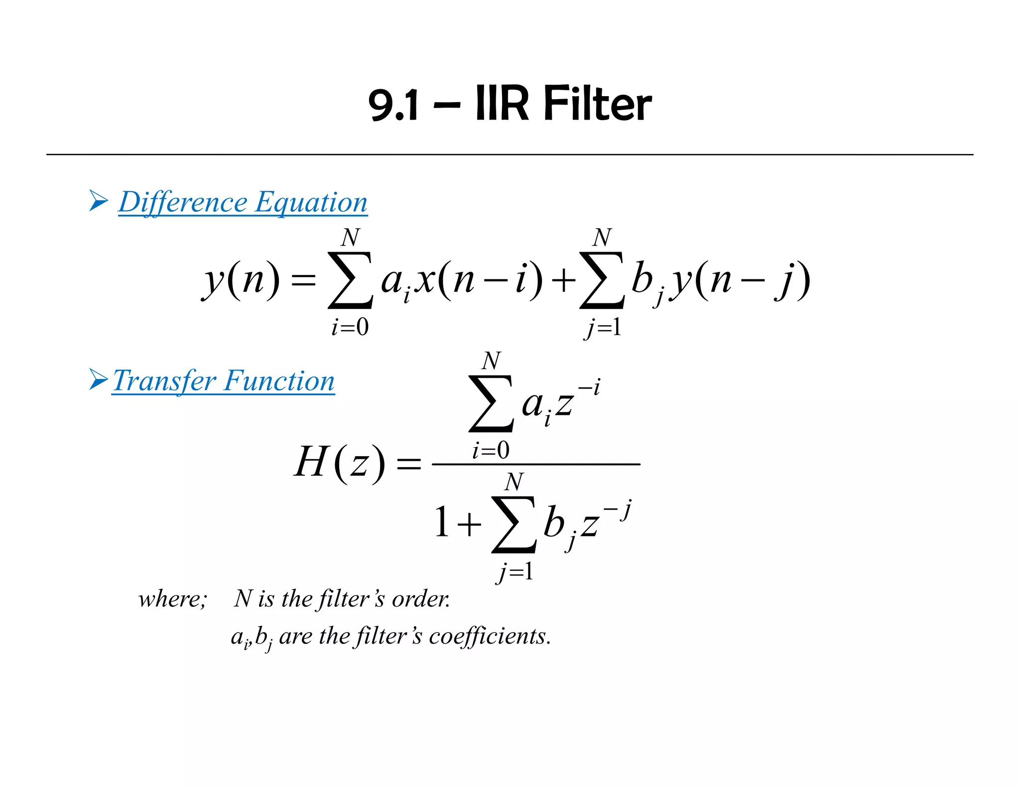
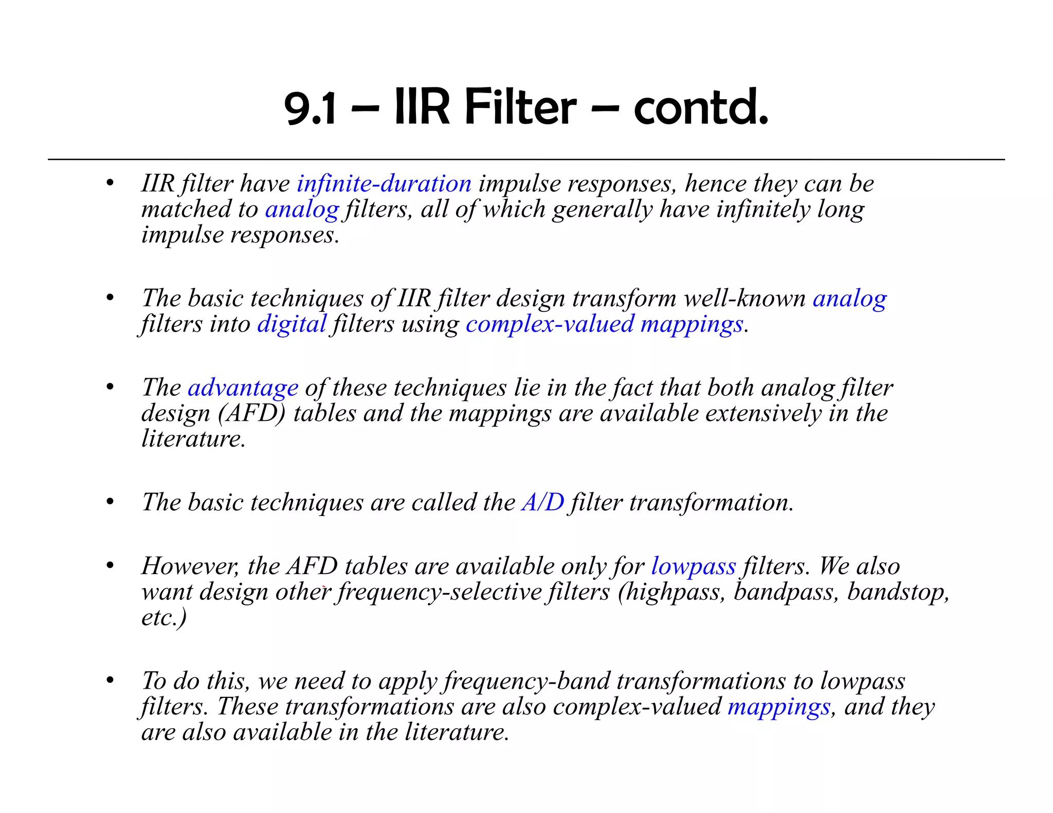
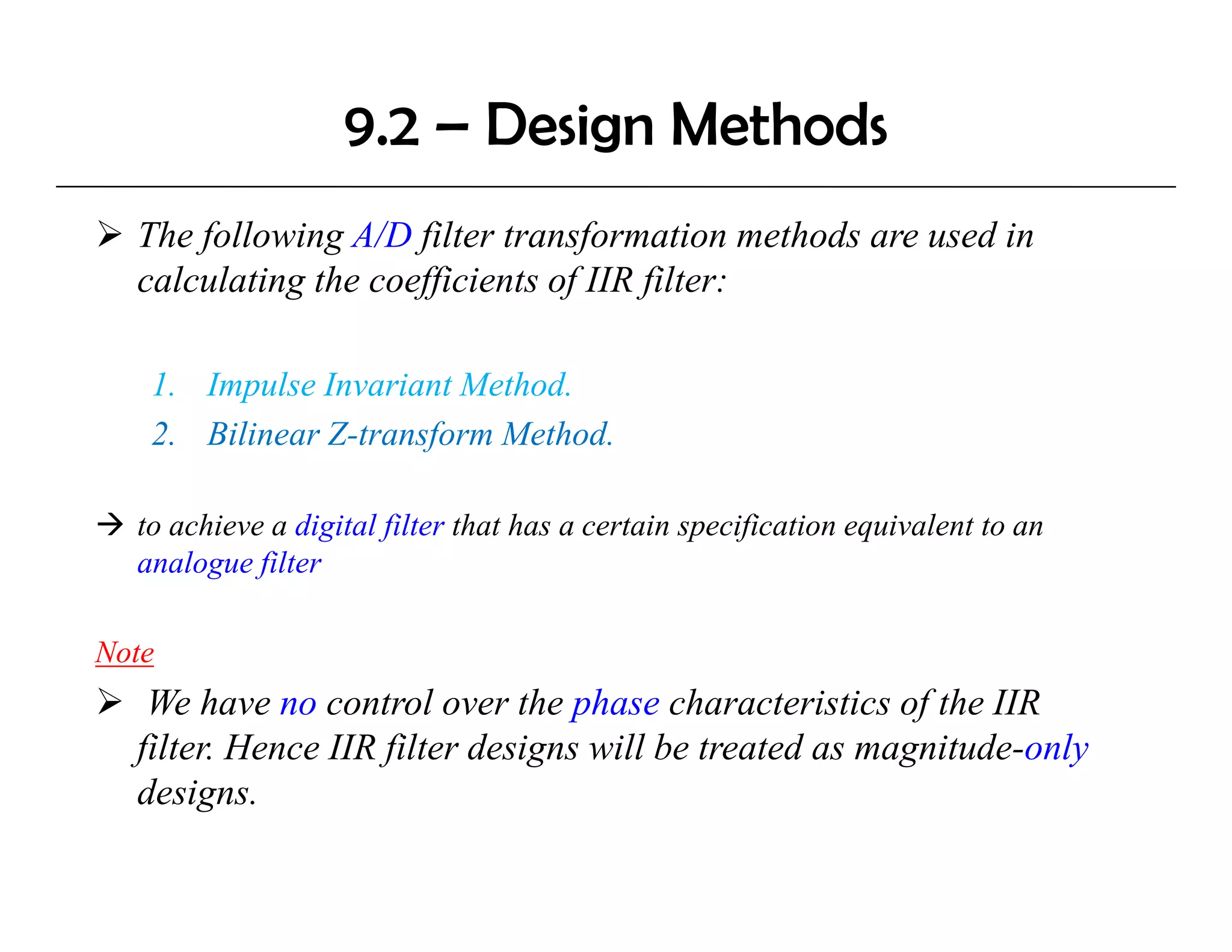
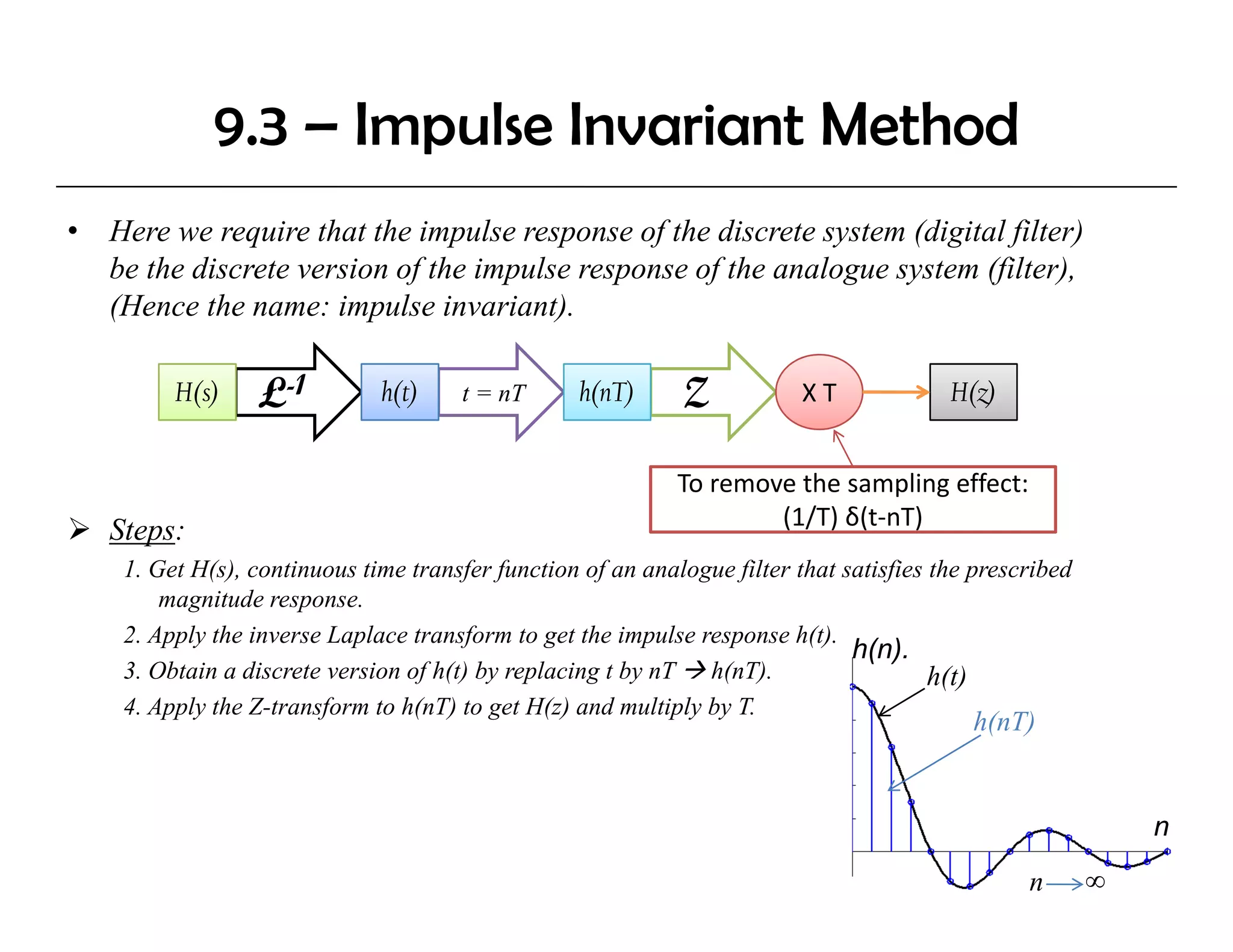
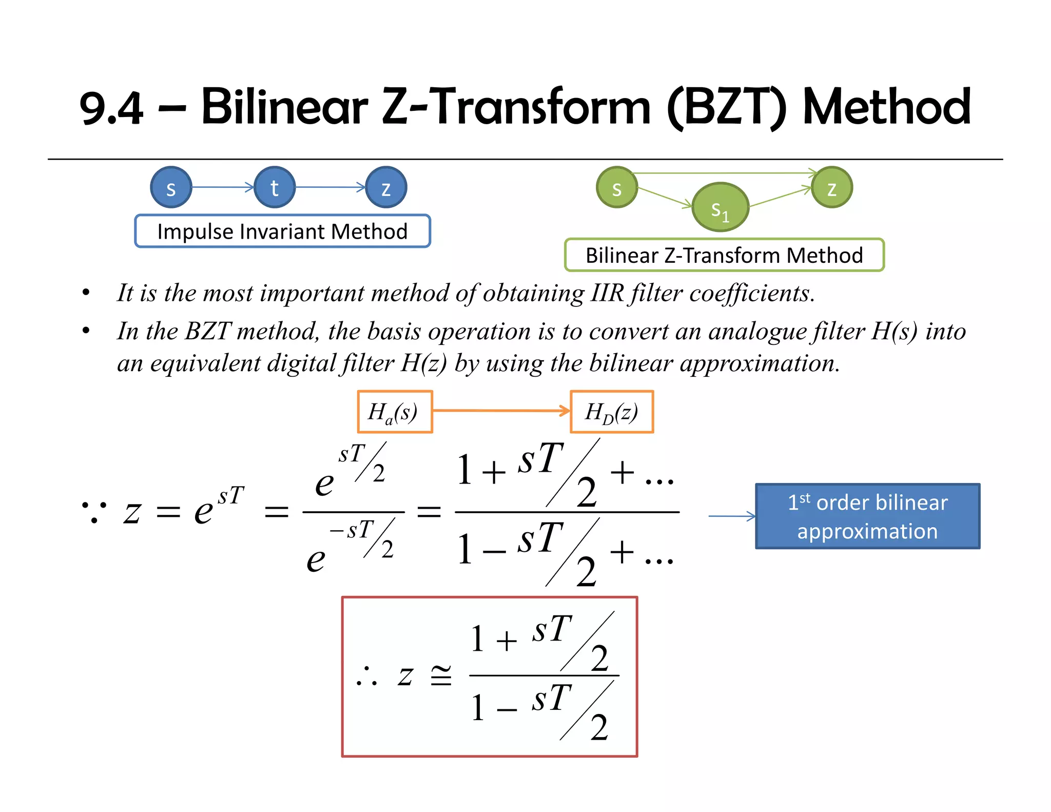
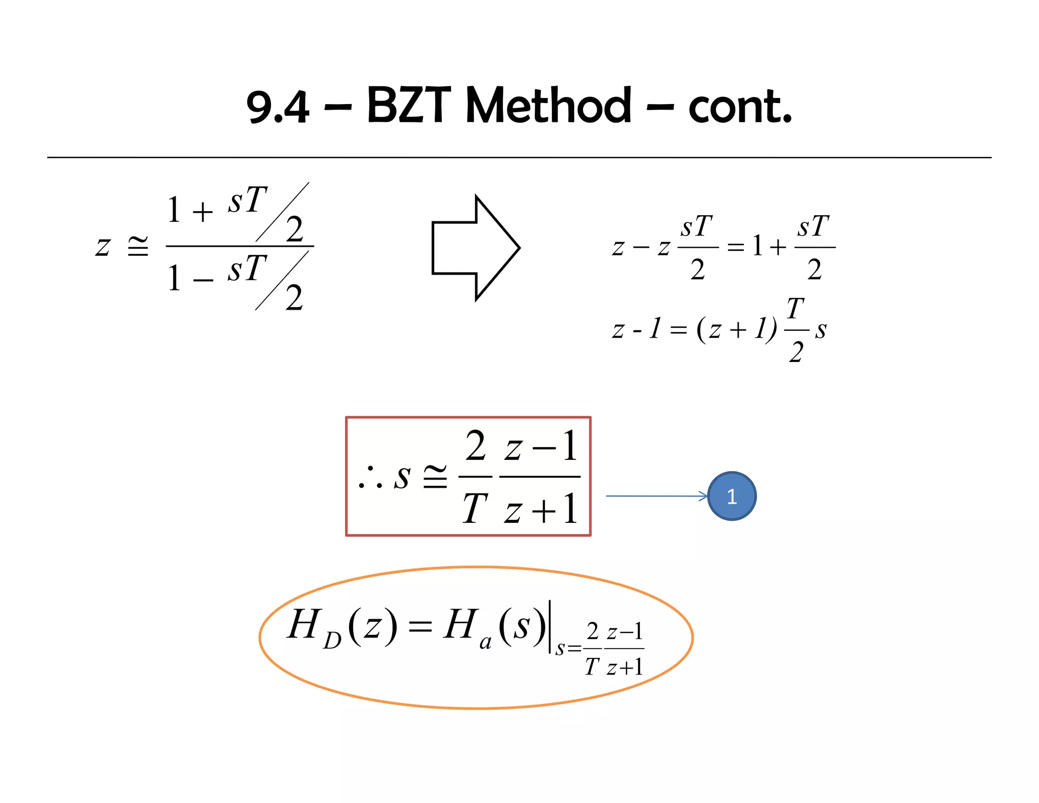
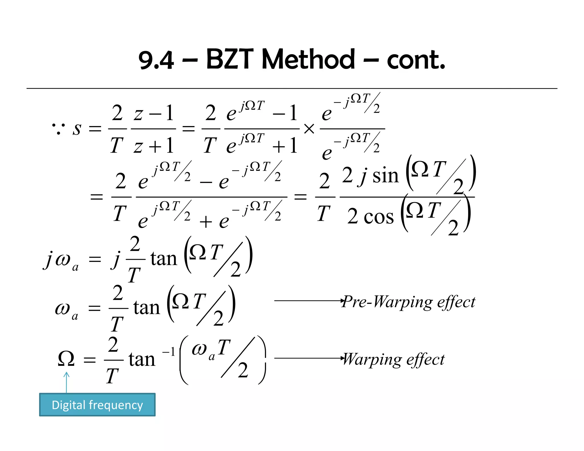
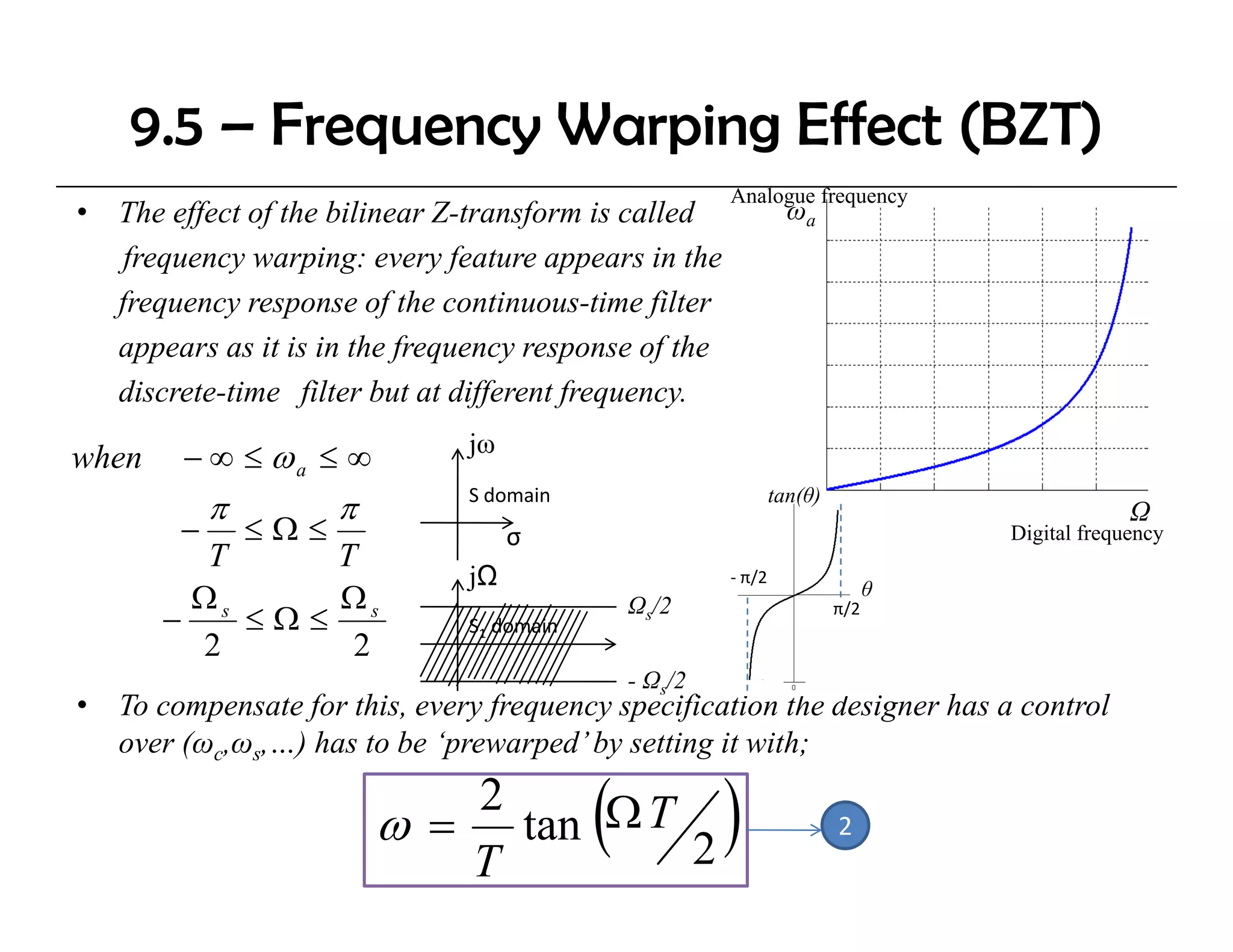
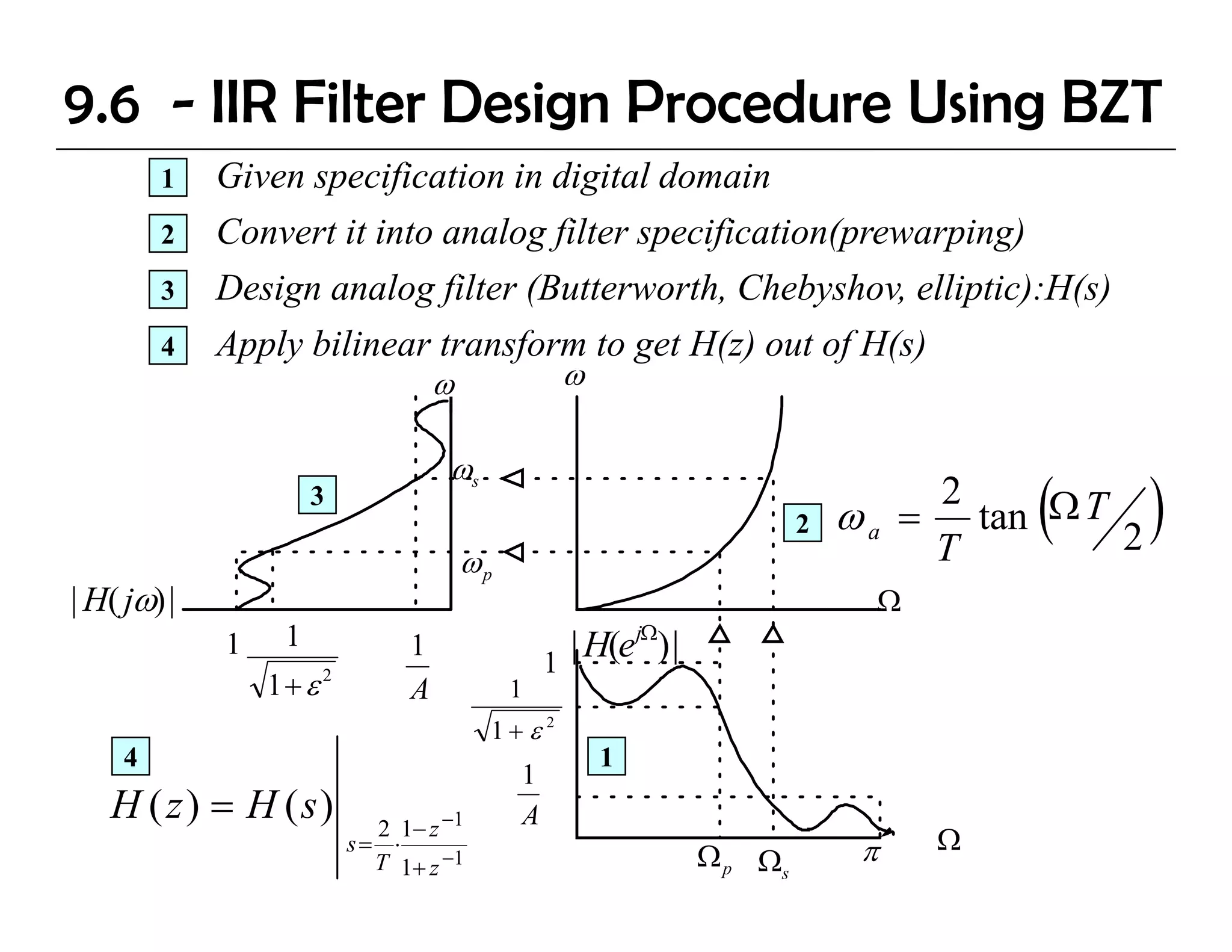
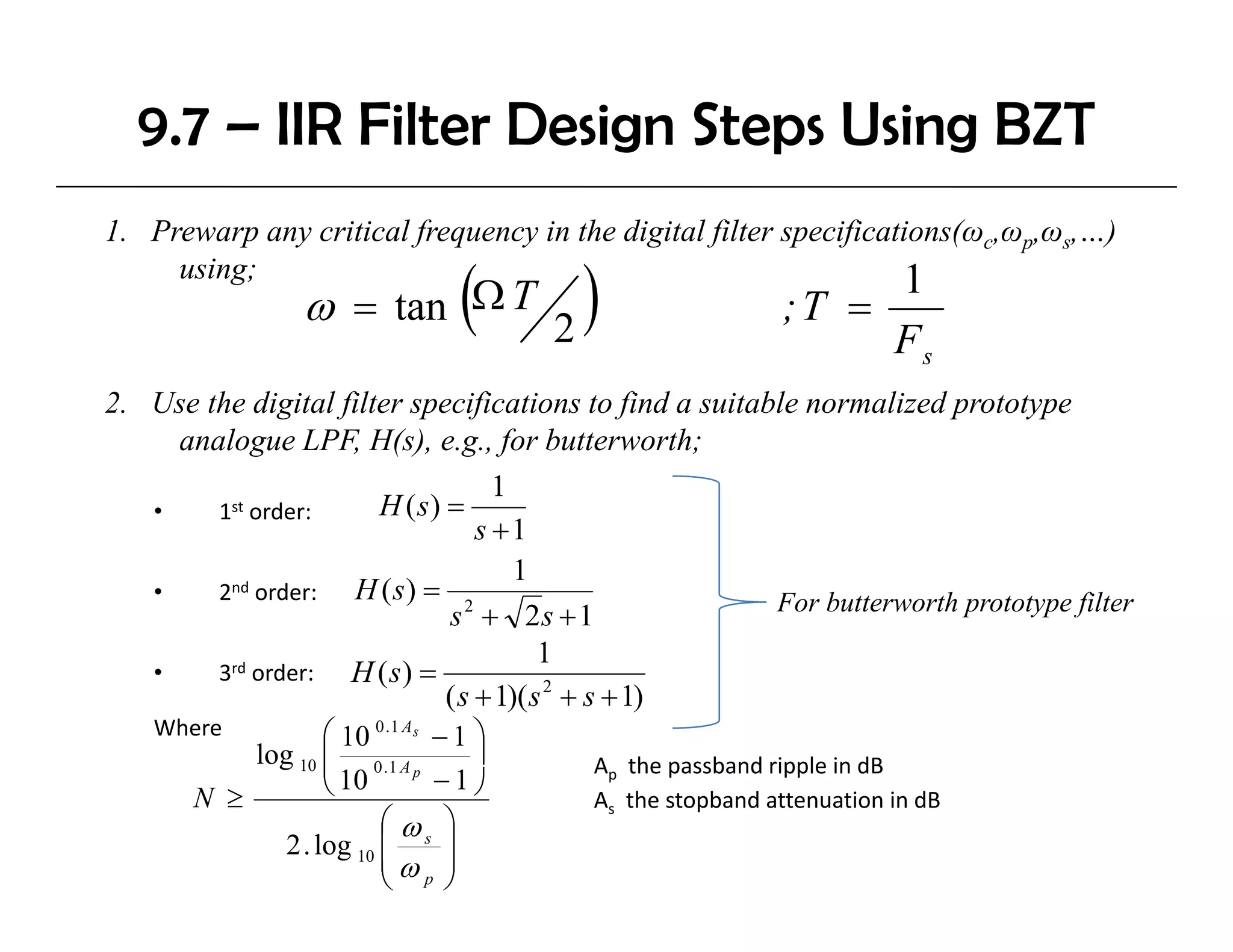
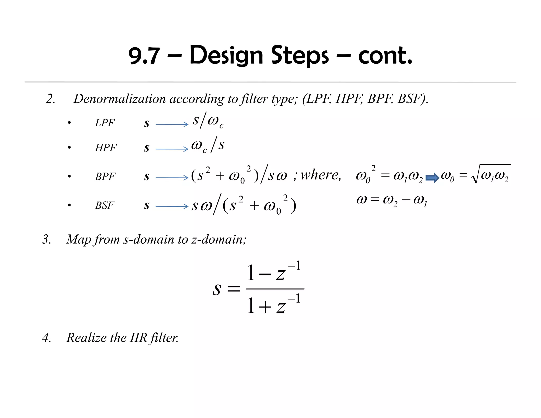
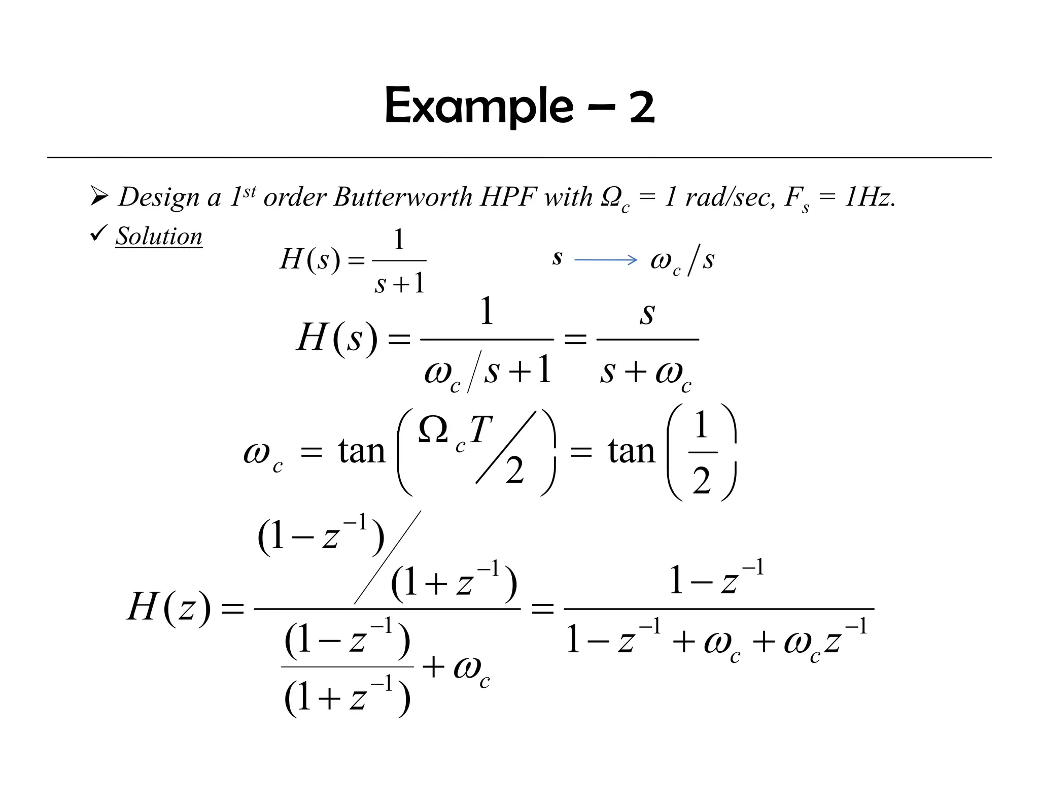
The document discusses the design of IIR digital filters using different methods. It begins by describing the difference equation and transfer function of IIR filters. It then covers the Impulse Invariant Method and Bilinear Z-Transform (BZT) Method for designing IIR filters by transforming analog prototypes. Key steps include prewarping frequencies, designing analog filters, and applying the bilinear transform. Examples demonstrate applying these methods to design Butterworth filters.

1. EC533: Digital Signal Processing
5 l l
Lecture 9
IIR Filter Design

2. 9.1 – IIR Filter
Difference Equation
N N
y (n) = ∑ ai x(n − i ) + ∑ b j y (n − j )
i =0 j =1
N
∑a z
Transfer Function −i
i
H ( z) = i =0
N
1+ ∑ bj z −j
j =1
where; N is the filter’s order.
ai,bj are the filter’s coefficients.
filter s

3. 9.1 – IIR Filter – contd.
• IIR filter have infinite-duration impulse responses, hence they can be
matched to analog filters, all of which generally have infinitely long
impulse responses.
• The basic techniques of IIR filter design transform well-known analog
filters into digital filters using complex-valued mappings.
• The advantage of these techniques lie in the fact that both analog filter
design (AFD) tables and the mappings are available extensively in the
literature.
• The basic techniques are called the A/D filter transformation.
• However, th AFD tables are available only for l
H the t bl il bl l f lowpass filt
filters. We also
W l
want design other frequency-selective filters (highpass, bandpass, bandstop,
etc.)
• To do this, we need to apply frequency-band transformations to lowpass
filters. These transformations are also complex-valued mappings, and they
are also available in the literature.

4. 9.2 – Design Methods
The following A/D filter transformation methods are used in
calculating the coefficients of IIR filter:
g ff f f
1. Impulse Invariant Method.
2. Bilinear Z-transform Method.
to achieve a digital filter that has a certain specification equivalent to an
g f p f q
analogue filter
Note
We have no control over the phase characteristics of the IIR
filter. Hence IIR filter designs will be treated as magnitude-only
designs.

5. 9.3 – Impulse Invariant Method
• Here we require that the impulse response of the discrete system (digital filter)
be the discrete version of the impulse response of the analogue system (filter),
(Hence the name: impulse invariant).
(H h l )
H(s) Ł-1 h(t) t = nT h(nT) Z X T H(z)
To remove the sampling effect:
(1/T) δ(t‐nT)
Steps:
1. Get H(s), continuous time transfer function of an analogue filter that satisfies the prescribed
magnitude response.
2. Apply the inverse Laplace transform to get the impulse response h(t).
h(n).
3. Obtain a discrete version of h(t) by replacing t by nT h(nT). h(t)
4. Apply the Z-transform to h(nT) to get H(z) and multiply by T.
h(nT)
n
n ∞

6. Example - 1
Using the invariant impulse response method, design a digital
filter that has the shown pole-zero distribution. jω
x ω0
Solution
s+a
H (s) = σ
[ s + ( a + jω 0 )][ s + ( a − jω 0 )] ‐a
s+a
H (s) = x - ω0
[( s + a ) + ω 0 )]
2 2
−1
(1) L {H ( s)} = e − at
cos(ω0t ) = h(t )
(2) h(nT) = e − anT
cos(ω0 nT )
1 − e − aT cos( ω 0T ) z −1
(
(3) T × Z{ h(nT)} = ×T
1 − 2e cos( ω 0T ) z + e
− aT −1 − 2 aT − 2
z
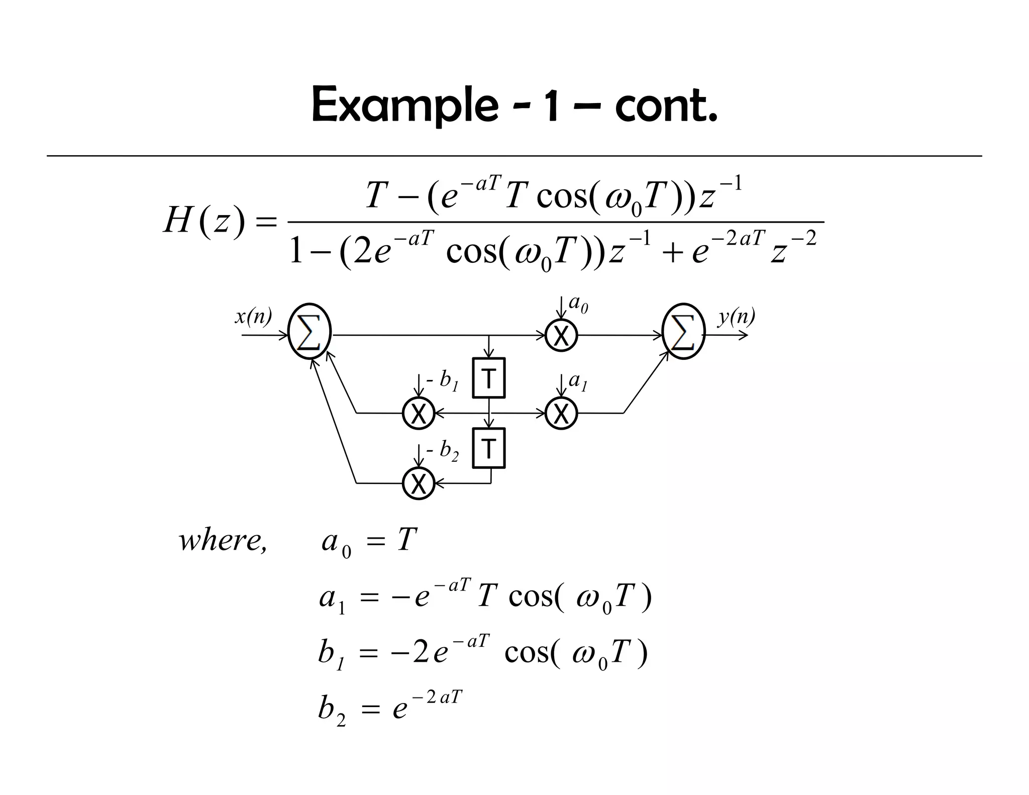
T − (e − aT T cos( ω 0T )) z −1
H ( z) =
1 − ( 2e − aT cos( ω 0T )) z −1 + e − 2 aT z − 2

7. Example - 1 – cont.
T − (e − aT T cos( ω 0T )) z −1
H ( z) =
1 − ( 2e − aT cos( ω 0T )) z −1 + e − 2 aT z − 2
a0
x(n) y(n)
X
- b1 T a1
X X
- b2 T
X
where, a0 = T
a 1 = − e − aT T cos( ω 0 T )
b1 = − 2 e − aT cos( ω 0 T )
b 2 = e − 2 aT

8. 9.4 – Bilinear Z-Transform (BZT) Method
s t z s z
s1
Impulse Invariant Method
Bilinear Z‐Transform Method
Bilinear Z Transform Method
• It is the most important method of obtaining IIR filter coefficients.
• In the BZT method, the basis operation is to convert an analogue filter H(s) into
an equivalent digital filter H( ) by using the bilinear approximation.
i l di i l fil H(z) b i h bili i i
Ha(s) HD(z)
1 + sT
sT
e 2 + ...
Qz =e sT
= = 2 1st order bilinear
− sT
1 − sT + ...
approximation
e 2
2
1 + sT
∴ z ≅ 2
1 − sT
2

9. 9.4 – BZT Method – cont.
1 + sT
z ≅ 2 z−z
sT
= 1+
sT
1 − sT 2 2
2 T
z - 1 = ( z + 1) s
2
2 z −1
∴s ≅
T z +1 1
H D ( z ) = H a ( s ) s = 2 z −1
T z +1

10. 9.4 – BZT Method – cont.
jΩ T − j ΩT
2 z −1 2 e −1 e 2
Qs = = jΩ T
× − j ΩT
T z +1 T e +1 e
( )
2
2 e
jΩT
2
−e
− jΩT
2
2 2 j sin Ω T
= = 2
T e j Ω T 2 + e − j Ω T 2 T 2 cos Ω T ( 2
)
2
jω a = j t Ω T
T
tan (2
)
2
ω a = tan Ω T 2
T
( ) Pre-Warping effect
p g ff
2 −1 ⎛ ω a T ⎞
Ω = tan ⎜ Warping effect
p g ff
T ⎝ 2 ⎠
Digital frequency

11. 9.5 – Frequency Warping Effect (BZT)
Analogue frequency
• The effect of the bilinear Z-transform is called ωa
frequency warping: every feature appears in the
frequency response of the continuous-time filter
f f th ti ti filt
appears as it is in the frequency response of the
discrete-time filter but at different frequency.
jω
when − ∞ ≤ ωa ≤ ∞
tan(θ)
π π S domain
Ω
− ≤Ω≤ σ Digital frequency
T T
jΩ ‐ π/2
Ωs Ωs Ωs/2
θ
− ≤Ω≤ S1 domain
π/2
2 2
- Ωs/2
• To compensate for this, every frequency specification the designer has a control
over (ωc,ωs,…) has to be ‘prewarped’ by setting it with;
2
ω = tan Ω T 2
T
( ) 2

12. 9.6 - IIR Filter Design Procedure Using BZT
1 Given specification in digital domain
2 Convert it into analog filter specification(prewarping)
3 Design analog filter (Butterworth, Chebyshov, elliptic):H(s)
(Butterworth Chebyshov
4 Apply bilinear transform to get H(z) out of H(s)
ω ω
ωs
3
2
2
(
ω a = tan Ω T 2
T
)
ωp
| H( jω) | Ω
1 1 1
1
| H(ejΩ) |
1+ ε 2 A 1
1+ε2
4 1
1
H ( z ) = H (s) 2 1− z −1 A
s= ⋅ π Ω
T 1 + z −1 Ω p Ωs

13. 9.7 – IIR Filter Design Steps Using BZT
1. Prewarp any critical frequency in the digital filter specifications(ωc,ωp,ωs,…)
( )
using; 1
ω = t ΩT 2
tan ;T =
Fs
2. Use the digital filter specifications to find a suitable normalized prototype
g f p f f p yp
analogue LPF, H(s), e.g., for butterworth;
1
• 1st order: H (s) =
s +1
1
• 2nd order: H (s) = 2 For butterworth prototype filter
s + 2s + 1
1
• 3rd order: H ( s ) =
( s + 1)( s 2 + s + 1)
Where ⎛ 10 0 .1 As − 1 ⎞
log 10 ⎜ 0 .1 A p
⎜ 10 ⎟ Ap the passband ripple in dB
p pp
⎝ −1⎠ p
N ≥ As the stopband attenuation in dB
⎛ ωs ⎞
2 . log 10 ⎜ ⎟
⎜ω ⎟
⎝ p⎠

14. 9.7 – Design Steps – cont.
2. Denormalization according to filter type; (LPF, HPF, BPF, BSF).
• LPF s s ωc
• HPF s ωc s
( s 2 + ω 0 ) s ω ; where, ω0 = ω1ω2 ω0 = ω1ω2
2 2
• BPF s
• BSF s sω ( s 2 + ω )
2 ω = ω2 − ω1
0
3.
3 Map f
M from s-domain to z-domain;
d i d i
−1
1− z
s= −1
1+ z
4.
4 Realize the IIR filter.
filter

15. Example – 2
Design a 1st order Butterworth HPF with Ωc = 1 rad/sec, Fs = 1Hz.
Solution 1
H ( s) = s ωc s
s +1
1 s
H ( s) = =
ωc s +1 s + ωc
ω c = tan ⎜ ⎛ Ω c T ⎞ = tan ⎛ 1 ⎞
2 ⎠ ⎜
⎝ ⎝2⎠
−1
(1 − z )
−1
−1
(1 + z ) 1− z
H ( z) = =
−1
(1 − z ) 1 − z + ωc + ωc z
−1 −1
−1
+ ωc
(1 + z )

16. Example - 2 – cont.
1 1 − z −1
H ( z) = 1
1 + ωc 1 + ωc − 1 z −1 k=
1 + ωc
ωc + 1
k a0
x(n) y(n)
X X
- b1 T a1
X X
where, a0 = 1
a1 = − 1
ωc −1
b1 =
ωc + 1

17. Example - 3
Design a 3rd order Butterworth LPF to have a cutoff frequency at 4 kHz
using the BZT method & assuming a sampling frequency of 10 kHz.
Solution 1
f c = 4 kHz & T= = 10 − 4 sec
Fs
Ω cT = 2π × 4 × 103 × 10 −4 = 2.513 rad
Ω cT
prewarping : ωc = tan( ) = 3.0762 rad
2 sec
1
H (s) =
( s + 1)( s 2 + s + 1)
1
H ( z) =
⎛ 1 ⎛ 1 − z ⎞ ⎞⎜
−1 ⎛ ⎛ 1 ⎞ 2 ⎛ 1 − z −1 ⎞ 2 1 ⎛ 1 − z −1 ⎞ ⎞
⎜ ⎜ ⎜ 1 + z −1 + 1 ⎜ ⎜ ω ⎜ 1 + z −1 + ω ⎜ 1 + z −1 + 1⎟
⎜ ⎜ ⎜
⎜ω
⎝ c⎝ ⎠ ⎠⎝ ⎝ c ⎠ ⎝ ⎠ c ⎝ ⎠ ⎠

18. Example - 3 – cont.
−1 −1 2
(1+ z ) (1+ z )
H(z) =
(
(1.3249+ 0.6751z−1) 0.105 (1− z−1)2 + 0.3249(1− z−2 ) + (1+ z−1)2 )
(1 + z − 1 ) (1 + 2 z − 1 + z − 2 )
=
1 . 3249 (
(1 + 0 .5095 z −1 ) 1.4305 + 1.789 z −1 + 0 .7806 z − 2 )
(1 + z − 1 ) (1 + 2 z − 1 + z − 2 )
= ×
(
1 . 3249 (1 + 0 .5095 z ) 1 . 4305 1 + 1 . 2506 z −1 + 0 . 5457 z − 2
−1
)
(1 + z − 1 ) (1 + 2 z − 1 + z − 2 )
= 0 . 52763 × ×
(
(1 + 0 .5095 z ) 1 + 1 . 2506 z −1 + 0 . 5457 z − 2
−1
)

19. Example - 3 – cont.
Filter Realization (Cascaded Realization)
0.52763
0 52763
x(n) X y(n)
- 0.5095 - 1.2506 2
T T
X X X
- 0.5457
T
X

20. Example - 4
Using BZT method, design a digital filter meeting the specifications
given by the following tolerance structure, |H(f)|
assume a Butterworth characteristic for this 1
filter. 0.707
Solution
0.1
f
(1) From the specifications, the prewarped frequencies are: 0.5 2 4 kHz
⎛ 2π × 500 ⎞
ω p = tan⎜ = 0.198912
⎝ 2 × 8000 ⎠
⎛ 2π × 2000 ⎞
ωs = tan⎜ =1
⎝ 2 × 8000 ⎠

21. Example - 4 – contd.
(2) D t
Determine th order of th prototype analogue B tt
i the d f the t t l Butterworth LPF using th f ll i
th i the following
relation,
⎛ 1 ⎞
⎜ −1 ⎟
⎜ δs
2
log ⎛ As 10 ⎞
⎜ 1 ⎟ log ⎜ 10 −1 ⎟
−1⎟ ⎜ Ap
⎜
(1 − δ p ) 2 ⎜ 10 10 − 1 ⎟⎟
N≥ ⎝ ⎠= ⎝ ⎠
⎛ ωs ⎞ ⎛ ωs ⎞
2 × log ⎜ ⎟ 2 × log ⎜ ⎟
⎜ω ⎟ ⎜ω ⎟
⎝ p ⎠ ⎝ p⎠
1 1 1 ⎛ 99 ⎞
−1 = − 1 = 99 , − 1 = 2 − 1 = 1 ⇒ log⎜ ⎟ = 1.995635
δs2 0.01 (1 − δ p ) 2 ⎝ 1 ⎠
⎛ ωs ⎞
2 × log⎜ ⎟ = 2 × log⎛
⎜
1 ⎞
⎟ = 1.402678
⎜ω ⎟ ⎝ 0.198912 ⎠
⎝ p⎠
1.995635
N≥ = 1.423. Let N = 2
1.402678

22. Example - 4 – contd.
(3) A 2nd order B tt
d Butterworth analogue LPF has the s-plane transfer function, H(s), given by,
th l h th l t f f ti H( ) i b
1
H (s) = 2
s + 2s + 1
(4) For a denormalized LPF transfer function, substitute s s ωp
1 ωp 2
H (s) = =
s 2 + 2 sω p + ω p
2 2
⎛ s ⎞
⎜ ⎟ + 2 s +1
⎜ω ⎟ ωp
⎝ p ⎠
(5) Applying the BZT,
ωp2
H ( z ) = H ( s ) s =⎜ 1− z −1 ⎟ =
⎛ ⎞
2
⎜ 1+ z −1 ⎟
⎝ ⎠ ⎛ 1− z ⎞ −1
⎛ 1 − z −1 ⎞
⎜ 1 + z −1 ⎟ + 2 ω p ⎜ 1 + z −1 ⎟ + ω p
2
⎜ ⎜
⎝ ⎠ ⎝ ⎠
ω p (1 + z −1 )
2 2
=
(1− z ) +
−1 2
(
2 ωp 1− z −1
)(1+ z )+ ω (1+ z )
−1
p
2 −1 2

23. Example - 4 – contd.
ω p (1 + 2z −1 + z −2 )
2
H ( z) =
(1− 2z −1
+z −2
)+ 2 ω (1 − z ) + ω (1 + 2z
p
−2
p
2 −1
+z −2
)
ω p 2 (1 + 2 z −1 + z −2 )
H ( z) =
(1 + 2 ω p + ω p ) + 2 (ω p − 1) z + (1 − 2 ω p + ω p ) z −2
2 2 −1 2
Substituting the values of the parameters,
g f p
1 + 2 ω p + ω p = 1.32087 , ω p − 1 = −0.96043
2 2
1 − 2 ω p + ω p = 0.7582858 , ω p = 0.0395659
2 2
H (z) =
0 .0395659 1 + 2 z + z ( −1 −2
)
1 .32087 − 1 .92086 z −1 + 0 .7582858 z − 2

24. Example - 4 – contd.
Dividing top & buttom by (1 + 2 ω p + ω p ) = 1 .32087
2
H (z) =
(
0 .02995 1 + 2 z − 1 + z − 2 )
−1 −2
1 − 1 .4542 z + 0 .57408 z
k a0
(6) Realization
Realization, x(n) y(n)
X X
- b1 T a1
X X
- b2 T a2
X X
where, k = 0 . 02995
a 0 = 1 , a1 = 2 , a 2 = 1
b1 = − 1 . 4542 , b 2 = 0 . 57408