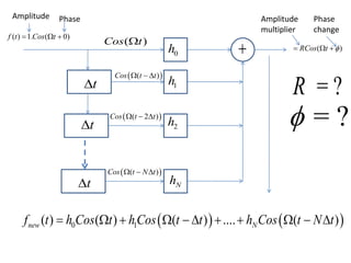
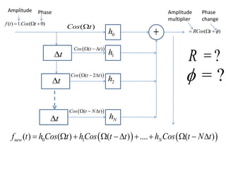
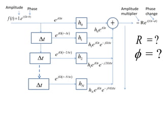
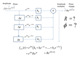
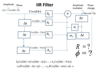
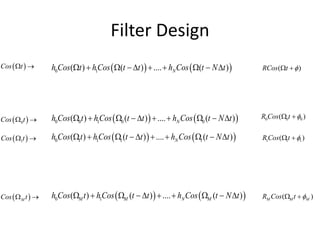
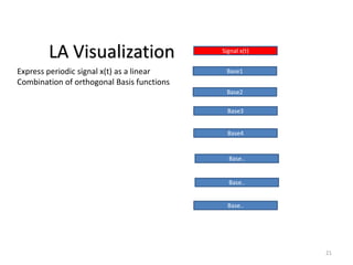
This document discusses linear algebra concepts for digital filter design. It begins with definitions of filters and digital filters, then covers topics like FIR and IIR filter design. Key points include: - A filter removes unwanted things from an item of interest passed through a structure. A digital filter removes unwanted frequency components from a discretized signal passed through a structure with delay, multiplier, and summer elements. 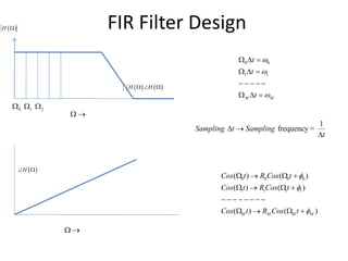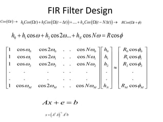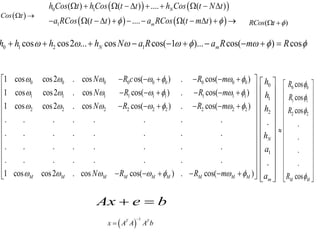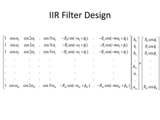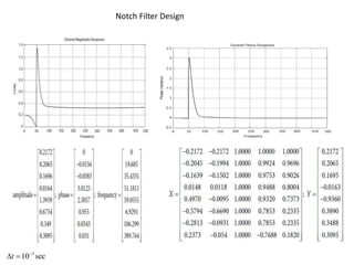- FIR filter design involves choosing filter coefficients to satisfy desired frequency response specifications. IIR filter design similarly involves solving systems of equations to determine coefficients for structures using feedback. - Matlab code for FIR filter design is provided in slide 17 for appreciation. A presentation on slides 3-4 and 17 is assigned.

1. Linear Algebra for Digital Filter
Design
Lecture Date: August 23
Presentation Assignment MIS3 5.3
for No:3 and 4 in each group.
Simply present these slides.
Matlab code for FIR filter design given in
Slide 17 will be appreciated
Date August 28 Evening

2. What is a filter?..
When an item of interest is passed through a structure/device
unwanted things are removed. That structure/device is called
Filter.

3. What is a Digital filter?..
When a discretized signal is passed through a structure
(consisting of delay , multiplier and summer elements)
unwanted frequency components are removed.
Generally the ordered sequence of multiplier elements
are called digital filter.

4. ( )Cos t
t
t
t
0h
Nh
1h
2h

 ( )Cos t t  
 ( 2 )Cos t t  
 ( )Cos t N t  
   0 1( ) ( ) ( ) .... ( )new Nf t h Cos t hCos t t h Cos t N t          
( )RCos t   
= ?R
= ?
( ) 1. ( 0)f t Cos t  
Amplitude Phase Amplitude
multiplier
Phase
change

5. ( )Cos t
t
t
t
0h
Nh
1h
2h

 ( )Cos t t  
 ( 2 )Cos t t  
 ( )Cos t N t  
   0 1( ) ( ) ( ) .... ( )new Nf t h Cos t hCos t t h Cos t N t          
( )RCos t   
= ?R
= ?
( ) 1. ( 0)f t Cos t  
Amplitude Phase Amplitude
multiplier
Phase
change

6. j t
e 
t
t
t
0h
Nh
1h
2h

 j t t
e  
 
Re j t  

= ?R
= ?
( 0)
( ) 1. j t
f t e  

Amplitude Phase Amplitude
multiplier
Phase
change
1
j t j t
h e e  
j t jN t
Nh e e  
 2j t t
e   
 j t N t
e   
0
j t
h e 
2
1
j t j t
h e e  

7. j t
e 
t
t
t
0h
Nh
1h
2h

j t j
e e  
 0 1( ) ....j t j jN
new Nf t e h he h e   
   
 
Rej t  

= ?R
= ?
( 0)
( ) 1. j t
f t e  

Amplitude Phase Amplitude
multiplier
Phase
change
2j t j
e e  
j t jN
e e  
ej t j
e R 

 j t
Re  


8. DTFT
0 1 .... ej jN j
Nh h e h e R   
   
Why we call it as DTFT?.

9. Consider a non periodic function h(t)
that exist for a short interval.
0
0 0
the domain of function h(.) be time 0 to T.
FT is
( ) ( ) ( )
on discretization of of time t in to n t, n=0,1,..,N
( t) ( )
t T
i t i t
t t
N N
i n t i
n n
Let
Its
H h t e dt h t e dt
h n e h n e

   
 
    
 
  
 

 
 @
2
2
0 1 2
= ( ), ,
(0) (1) (2) .... ( )
, equivalently H( )= ....
n
i i iN
i i iN
N
H t
h h e h e h N e
Or h h e h e h e

  
  
 

  
  
 
    
   

10. ( )Cos t
t
t
t
0h
Nh
1h
2h

 ( )Cos t t  
 ( 2 )Cos t t  
 ( )Cos t N t  
( )RCos t   
= ?R
= ?
( ) 1. ( 0)f t Cos t  
Amplitude Phase Amplitude
multiplier
Phase
change
IIR Filter
t
1a
2a t
   
   
0 1
1
( ) ( ) .... ( )
( ) .... ( )
N
m
h Cos t hCos t t h Cos t N t
a RCos t t a RCos t m t 
         
           

11. FIR Filter Design
0 1 2
0 0
1 1
M M
t
t
t



  
  
    
  
0 0 0 0
1 1 1 1
( ) ( )
( ) ( )
( ) ( )M M M M
Cos t R Cos t
Cos t R Cos t
Cos t R Cos t



   
   
       
   
1
frequency =Sampling t Sampling
t
 

   H H  
 H 
 
 
 H 

12. Filter Design
   0 1( ) ( ) .... ( )Nh Cos t hCos t t h Cos t N t          ( )RCos t  
   0 1 1 1 1( ) ( ) .... ( )Nh Cos t hCos t t h Cos t N t          1 1 1( )R Cos t  
   0 0 1 0 0( ) ( ) .... ( )Nh Cos t hCos t t h Cos t N t          0 0 0( )R Cos t  
   0 1( ) ( ) .... ( )M M N Mh Cos t hCos t t h Cos t N t          ( )M M MR Cos t  
 0Cos t 
 1Cos t 
 MCos t 
 Cos t 

13. FIR Filter Design
 Cos t     0 1( ) ( ) .... ( )Nh Cos t hCos t t h Cos t N t           ( )RCos t  
0 1 2cos cos2 ... cos cosNh h h h N R      
00 0 0 0 0
11 1 1 1 1
22 2 2 2 2
1 cos cos2 . . cos cos
1 cos cos2 . . cos cos
1 cos cos2 . . cos cos
.. . . . . . .
.. . . . . . .
1 cos cos2 . . cos cosNM M M M M
hN R
hN R
hN R
hN R
   
   
   
   
    
    
    
    
    
    
    
    
    
Ax e b 
 
1T T
x A A A b



14. IIR Filter design

15.  Cos t 
   
   
0 1
1
( ) ( ) .... ( )
( ) .... ( )
N
m
h Cos t hCos t t h Cos t N t
a RCos t t a RCos t m t 
         
            ( )RCos t  
0 1 2 1cos cos2 ... cos cos( 1 )... cos( ) cosN mh h h h N a R a R m R                
Ax e b 
 
1T T
x A A A b


0 0 0 0 0 0 0 0 0
1 1 1 1 1 1 1 1 1
2 2 2 2 2 2 2 2 2
1 cos cos2 . cos os( ) . cos( )
1 cos cos2 . cos cos( ) . cos( )
1 cos cos2 . cos cos( ) . cos( )
. . . . . . . .
. . . . . . . .
. . . . . . . .
. . . . . . . .
1 cos cos2 . cosM M M
N R c R m
N R R m
N R R m
N R
      
      
      
  
     
     
     
 cos( ) . cos( )M M M M M MR m   
 
 
 
 
 
 
 
 
 
 
 
      
0
1
2
1
.
.
N
m
h
h
h
h
a
a
 
 
 
 
 
 
 
 
 
 
 
  
0 0
1 1
2 2
cos
cos
cos
.
.
.
.
cosM M
R
R
R
R




 
 
 
 
 
 
 
 
 
 
 
  

16. IIR Filter Design
0 0 0 0 0 0 0 0 0
1 1 1 1 1 1 1 1 1
2 2 2 2 2 2 2 2 2
1 cos cos2 . cos os( ) . cos( )
1 cos cos2 . cos cos( ) . cos( )
1 cos cos2 . cos cos( ) . cos( )
. . . . . . . .
. . . . . . . .
. . . . . . . .
. . . . . . . .
1 cos cos2 . cosM M M
N R c R m
N R R m
N R R m
N R
      
      
      
  
     
     
     
 cos( ) . cos( )M M M M M MR m   
 
 
 
 
 
 
 
 
 
 
 
      
0
1
2
1
.
.
N
m
h
h
h
h
a
a
 
 
 
 
 
 
 
 
 
 
 
  
0 0
1 1
2 2
cos
cos
cos
.
.
.
.
cosM M
R
R
R
R




 
 
 
 
 
 
 
 
 
 
 
  

17. Notch Filter Design
3
10 sect 
 

18. Lecture over.
Remaining slides are for
Reference and for your
presentation

19. Everything you need to know
About Fourier family

20. FS FT
DTFT
DFT
Fourier Family

21. 21
LA Visualization Signal x(t)
Base1
Base2
Base3
Base4
Base..
Base..
Base..
Express periodic signal x(t) as a linear
Combination of orthogonal Basis functions

22. 2
1 1
2
0
2 21 1
0 0
2
( ) ,0 or ,
1
( )
on discretization of of time t in to n t, n=0,1,..(N-1)
( ) ( ) ( ) ( )
k i k t
T
k
k
T
i k t
T
k
t
N Ni k n t i k n
N t N
n n
x t X e t T t t t T
T
X x t e dt
T
X k x n e x n e x n


 
 

 

     

 
       

 
  


 
1
0
N
kn
N
n
W



FS
DFT
From Fourier series to DFT
k=0,1,2,…,N-1 Any N consecutive bases will do. Why?.
Not same.
Differ by a
scaling factor

23. From Fourier Transform to DTFT
1 1
0 0
( ) ( ) ( ) ; assume x is defined over 0 to T
on discretization of of time t in to n t, n=0,1,..(N-1)
( ) ( ) ( ) ,
(
t
i t i t
t t
N N
i n t i n
n n
X x t e dt x t e dt
X x n e x n e t
X

 


   

 
     
 
  
 
   
 
 
1 1
( 2 )
0 0
) is a continous function of but it is periodic with periodicity 2
( 2 ) ( ) ( )
N N
i n i n
n n
X x n e x n e  
 
 
 
    
 
   
Not same.
Differ by a
scaling factor
Note: x(t) need to be a time limited function for FT to exist

24. From FT to DFT via DTFT
1 1
0 0
( ) ( ) ( )
on discretization of of time t in to n t, n=0,1,..(N-1)
( ) ( ) ( ) , ,
( ) is periodic with period 2
on
t
i t i t
t t
N N
i n t i n
n n
X x t e dt x t e dt
X x n e x n e t
X

 
 

   

 
    
 
  
 
   

 
 
221 1 1
0 0 0
2
discretization of of from 0 to 2 in to , k=0,1,..(N-1)
X(k)= ( ) ( ) ( )
N N Ni kni k n
knNN
N
n n n
k
N
x n e x n e x n W


 
        
 
  
   
FT
DFT
2
is evaluation of X( ) at =kAbove
N

 

25. Create DFT matrix for N=8
0
1
2
3
4
5
6
7
8 DFT
bases are
e
e
e
0
e
2
e
e
e
e
i t
i t
i t
i t
i t
i t
i t
i t
The
t T
T

 
 
 
 
 
 
 
 




 


 





0
1
2
3
4
5
6
7
8 DFT conjugated
bases are
e
e
e
e
e
e
e
e
i t
i t
i t
i t
i t
i t
i t
i t
The
 
  
  
  
  
  
  
  
2 2
0 0
2
1
2
2
2
3
2
4
2
5
6
8 DFT conjugated
bases on sampling are
e e , 0,1, 2,.., 7
e , 0,1, 2,.., 7
e , 0,1, 2,.., 7
e , 0,1, 2,.., 7
e , 0,1, 2,.., 7
e , 0,1, 2,.., 7
e
n
i n t i
N t N
n
i
N
n
i
N
n
i
N
n
i
N
n
i
N
i
The
n
n
n
n
n
n
 





     

  
  
  
  
  
  
 





2
2
7
, 0,1, 2,.., 7
e , 0,1, 2,.., 7
n
N
n
i
N
n
n


  


2
Term for kth basis (starting from 0) is
, n=0,1,2,...,7
i
nk
nkN
N
Generic
e W




26. ?.
N property
Why
Mod
2 2
0 0
2
1
2
2
2
3
2
4
2
3
2
2
8 DFT conjugated
bases on sampling are
e e , 0,1, 2,..,7
e , 0,1, 2,..,7
e , 0,1, 2,..,7
e , 0,1, 2,..,7
e , 0,1, 2,..,7
e , 0,1, 2,..,7
e
n
i n t i
N t N
n
i
N
n
i
N
n
i
N
n
i
N
n
i
N
i
The
n
n
n
n
n
n
 






     

  
  
  
  
 
 
 





2
1
, 0,1, 2,..,7
e , 0,1, 2,..,7
n
N
n
i
N
n
n

 



27. 5 3
8 8W W , for int nn n
Why eger  
 
        mod N mod N k mod N n mod N mod
5 ( 5 mod 8) 3
8 8 8
Proof: We have the relation
W W W W W
W W =W , for int n
k n n k kn Nkn
N N N N N
n n n
eger    
   
 
6 2
8 8
7 1
8 8
W W , for int n
W W , for int n
n n
n n
Similarly
eger
eger
  
  
 
 

28.  
Angular Frequency is .
2
, T is the periodicity of the signal
If t from 0 to T is discretized to have N values, like
t=(0:N-1) t, t
t is now n t with n=0,1,2,..., N-1
T=N t
Fundamental
T
T
N
Generic


 
   


Details of Sampling
Signal is assumed to be periodic with period T
So, we sample signal from 0 to T
interval is t=Sampling
N



29. 0
T0 t 3 t2 t1 t
 1N t 
 2N t 
Sampling Instances
t 
Discretization: t=n t, n=0,1,2,3...,N-1After 
Generally index n is used for time
n varies from 0 to N-1
Index k is used for indexing the basis vector
k varies from 0 to N-1

30. 2 2
Term for kth basis (starting from 0) is
, n=0,1,2,...,7
i i
nk kn
knN N
N
Generic
e e W
  
 
 
k
0 0 0 1 0 2 0 3 0 4 0 5 0 6 0 7
1 0 1 1 1 1 1 3 1 4 1 5 1 6 1 7
2 0 2 1 2 2 2 3 2 4 2 5 2 6 2 7
3 0 3 1 3 2 3 3 3 4 3 5 3 6 3 7
4 0 4 1 4 2 4 3 4 4 4 5 4 6 4 7
N N N N N N N N
N N N N N N N N
N N N N N N N N
N N N N N N N N
N N N N N N N N
W W W W W W W W
W W W W W W W W
W W W W W W W W
W W W W W W W W
W W W W W W W W
       
       
       
       
       
5 0 5 1 5 2 5 3 5 4 5 5 5 6 5 7
6 0 6 1 6 2 6 3 6 4 6 5 6 6 6 7
7 0 7 1 7 2 7 3 7 4 7 5 7 6 7 7
N N N N N N N N
N N N N N N N N
N N N N N N N N
W W W W W W W W
W W W W W W W W
W W W W W W W W
       
       
       
 
 
 
 
 
 
 
 
 
 
  
 

31. Circular and Linear Convolution
     1 2
1 2
( ) ( ) ( ) , 0,1,2,.., 1
( ) ( ) ( ), 0,1,2,.., 1
y n x n x n n N
Y k X k X k k N
   
    
 
 
1
2
1 2
( ) is a long signal sequence of length N
( ) is a very short filter sequence padded with zeros up to N,
so that convolution is a linear convolution. Then
( ) ( ) ( ),
Suppose
x n
x n
Y k X k X k 
2
imply that filter sequence modify the
frequency content of the input signal upon convolution
( ) can be interpreted as filter response.
2
Corresponding to each k, there is a frequency, k
X k
T



32. Applications
1. Signal processing
2. Communication Engineering
3. Feature Extraction in ML