This document describes a global optimization technique for aligning multiple experiments of a modulated signal by correcting for phase offsets between them. The technique finds the delay and phase offset values that minimize the difference between the first experiment and each subsequent experiment. It is tested on a set of measurements of a field effect transistor's output current under a 3-tone modulated excitation. The results show improved alignment when correcting the experiments using the extracted delay and phase offset values.

1. Global optimization technique for phase de-trending
Global optimization technique for phase de-trending
G. Pailloncy, NMDG nv
Introduction
A modulated signal with a carrier frequency fc and presenting H harmonics can be represented by:
H
x t = ∑ a h t. e j 2 h f c t
(1)
h=−H
with ah(t), the modulating signal and a−h t =a ∗ t  , the complex conjugate of ah(t).
h
The modulating signal ah(t) is a complex signal that may be expressed in a general way as:
a h t =I h t− jQ h t (2)
In case of a modulating signal composed of 2N+1-tones and with a modulation frequency fm, ah(t) can be ex-
pressed as:
N
a h t = ∑ Ah , k e j2  k f m t
Ah , k ∈ℂ (3)
k =−N
When measuring with a sampler-based Large-Signal Network Analyzer (LSNA), such a modulated signal is
down-converted using a sampler. Due to the effect of the internal local oscillator (LO), a phase offset may oc-
curred Ф. Moreover, as no trigger is used when capturing the down-converted signal with the ADCs, a delay τ
may appear between the different measured experiments.
An i-th measured experiment can then be expressed as:
H N
x i t =x t− i , i =
 ∑ ∑ Ah ,k e− j2 h f c k f m i
e j h  e j2  h f
i c k f m t
(4)
h =−H k=− N
In the frequency domain, the modulated signal can be expressed as:
H N

X i  f = Fourier { x i t }∣ f =
 ∑ ∑ X i ,h , k   f −h f c k f m  (5)
h=−H k=−N
with
− j 2  h f c k f m i j h i
X i , h , k = Ah , k e e (6)
Our purpose, in this report, is to align the different experiments taking the first experiment x 0 t  as the refer-

ence (τ0 = 0, Ф0 = 0) by correcting for the delay τi and phase offset Фi between them.
© 2009 NMDG NV 1

2. Global optimization technique for phase de-trending
In the following, a global optimization technique to extract the delay τi and phase offset Фi is described and ap-
plied to a set of modulated signal measurements.
Correction of the delay and phase offset between experiments
The above equation (6) may be rewritten as:
X i , h , k = Ah , k e− j 2  k f e j h−2  f = Ah , k e− j 2  k f e j h
i  i i  i
m c m 0i
(7)
Applying a Least Square Estimator, the τi and Ф0i values that minimize the following function around the funda-
mental (h=1), need to be found for each experiment:
N
min S =
 i , 0i
∑  X 0,1, k − X i , 1,k e j2 k f m  i − j 0i
e  . X 0,1,k − X i ,1, k e j2  k f m i − j 0i ∗
e  (8)
k=−N
1 2 1
The function S is first computed for a set of 10 values both for τi ( [ , .. ] ) and for Ф0i (
10f m 10f m f m
1 2 1
[ , .. ] ) , and the pair of { τi, Ф0i} values that gives the minimum result is selected as initial
20  20  2 
guess values for the Least Square Estimator.
One may then correct each experiment for the delay and phase offset using the extracted τi and Ф0i:
X 'i , h , k = X i , h , k e j 2 k f i − j h0i
m
e (9)
Results
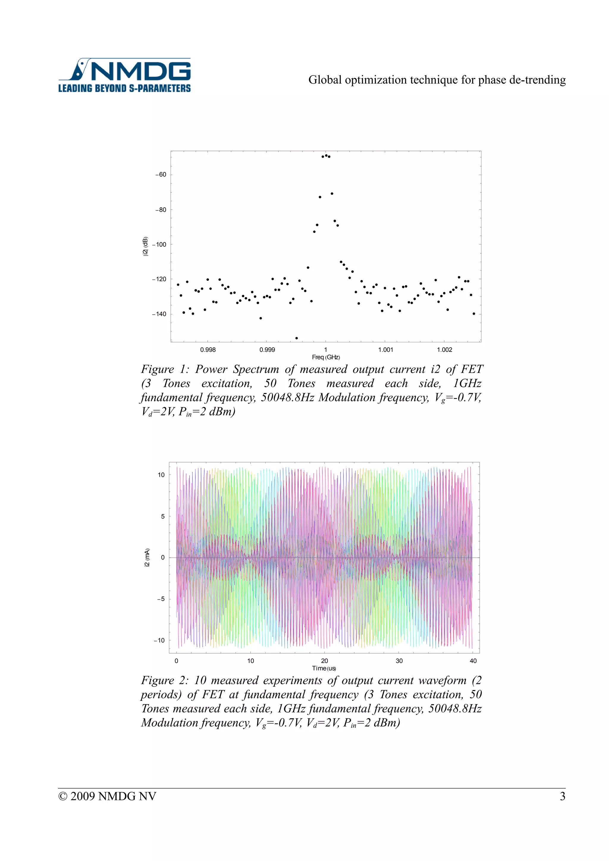
A set of 10 experiments of the measured output current of a commercially available FETis used. The FET is ex-
cited by a 3-Tones modulated signal with 1GHz fundamental frequency and 50048.8 Hz modulation frequency.
The power spectrum of the measured current is plotted on Figure 1.
The set of 10 experiments without any phase alignment is shown in time domain on Figure 2.
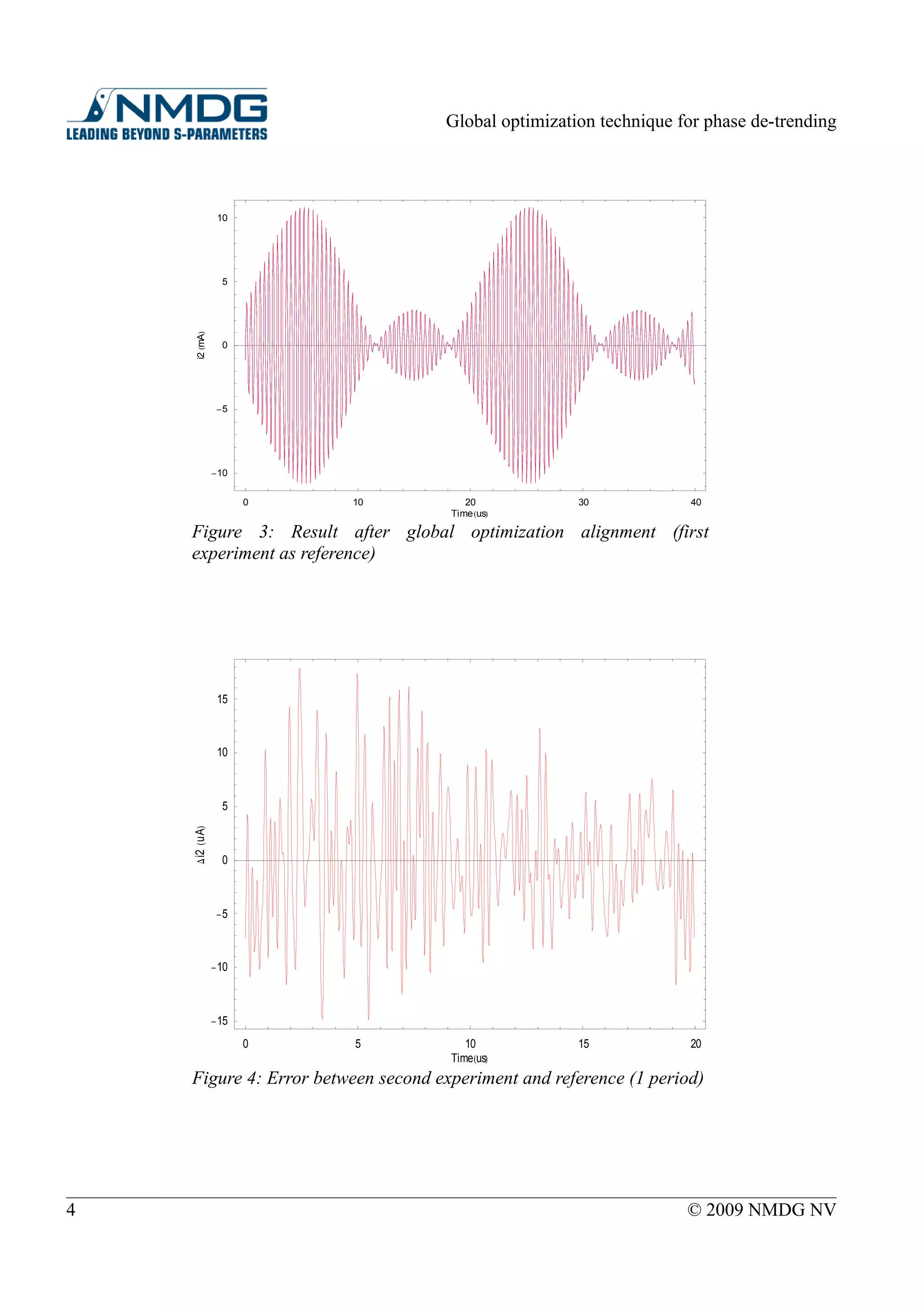
After applying the above global optimization technique with first experiment as reference, the results shown on
Figure 3.
To verify further the algorithm, the difference in time domain between the reference (first experiment) and the
aligned second experiment is plotted on Figure 4.
Conclusion
In this article,a global optimization technique to align a set of modulated signal experiments has been described
mathematically and tested.
2 © 2009 NMDG NV

3. Global optimization technique for phase de-trending
- 60
- 80
È i2È HdBL
- 100
- 120
- 140
Freq HGHzL
0.998 0.999 1 1.001 1.002
Figure 1: Power Spectrum of measured output current i2 of FET
(3 Tones excitation, 50 Tones measured each side, 1GHz
fundamental frequency, 50048.8Hz Modulation frequency, Vg=-0.7V,
Vd=2V, Pin=2 dBm)
10
5
i2 HmAL
0
-5
- 10
Time HusL
0 10 20 30 40
Figure 2: 10 measured experiments of output current waveform (2
periods) of FET at fundamental frequency (3 Tones excitation, 50
Tones measured each side, 1GHz fundamental frequency, 50048.8Hz
Modulation frequency, Vg=-0.7V, Vd=2V, Pin=2 dBm)
© 2009 NMDG NV 3

4. Global optimization technique for phase de-trending
10
5
i2 HmAL
0
-5
- 10
Time HusL
0 10 20 30 40
Figure 3: Result after global optimization alignment (first
experiment as reference)
15
10
5
D i2 H u AL
0
-5
- 10
- 15
Time HusL
0 5 10 15 20
Figure 4: Error between second experiment and reference (1 period)
4 © 2009 NMDG NV