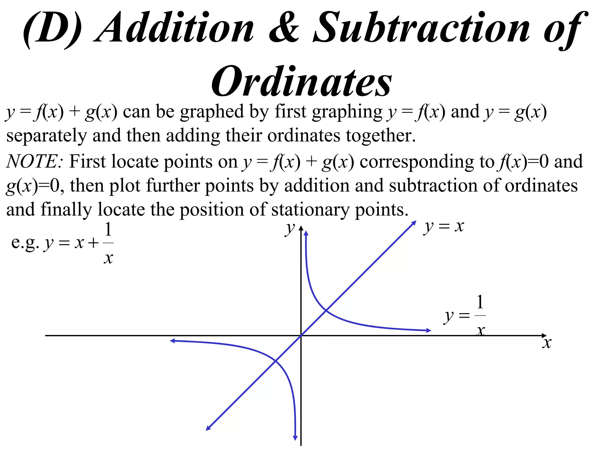
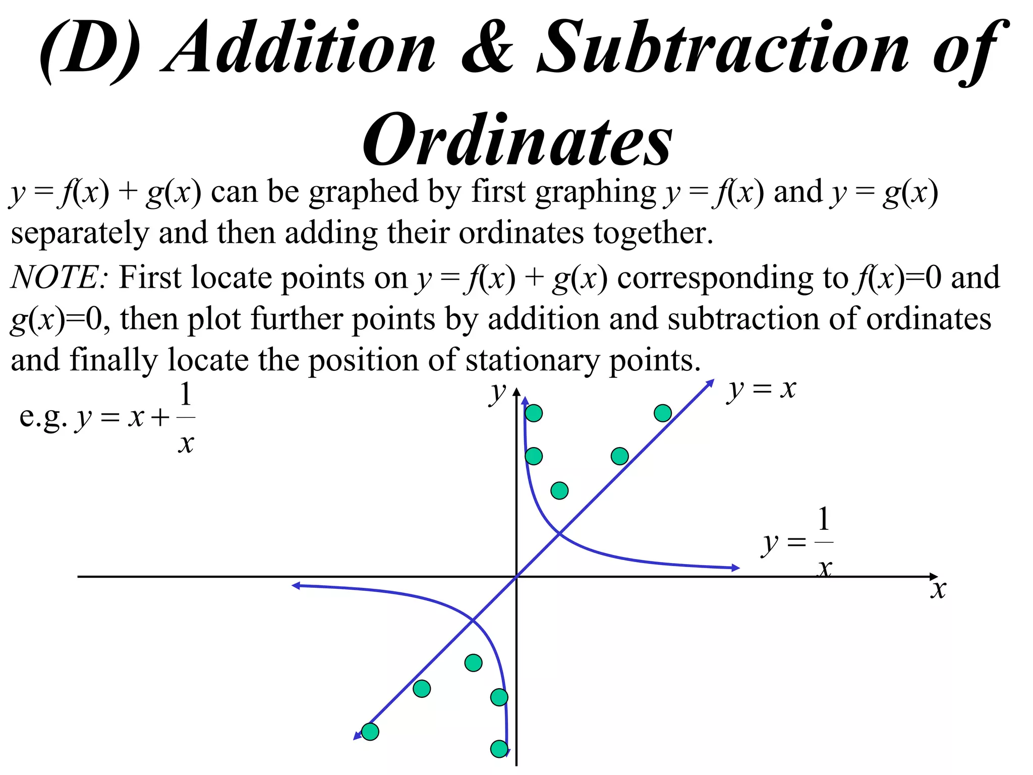
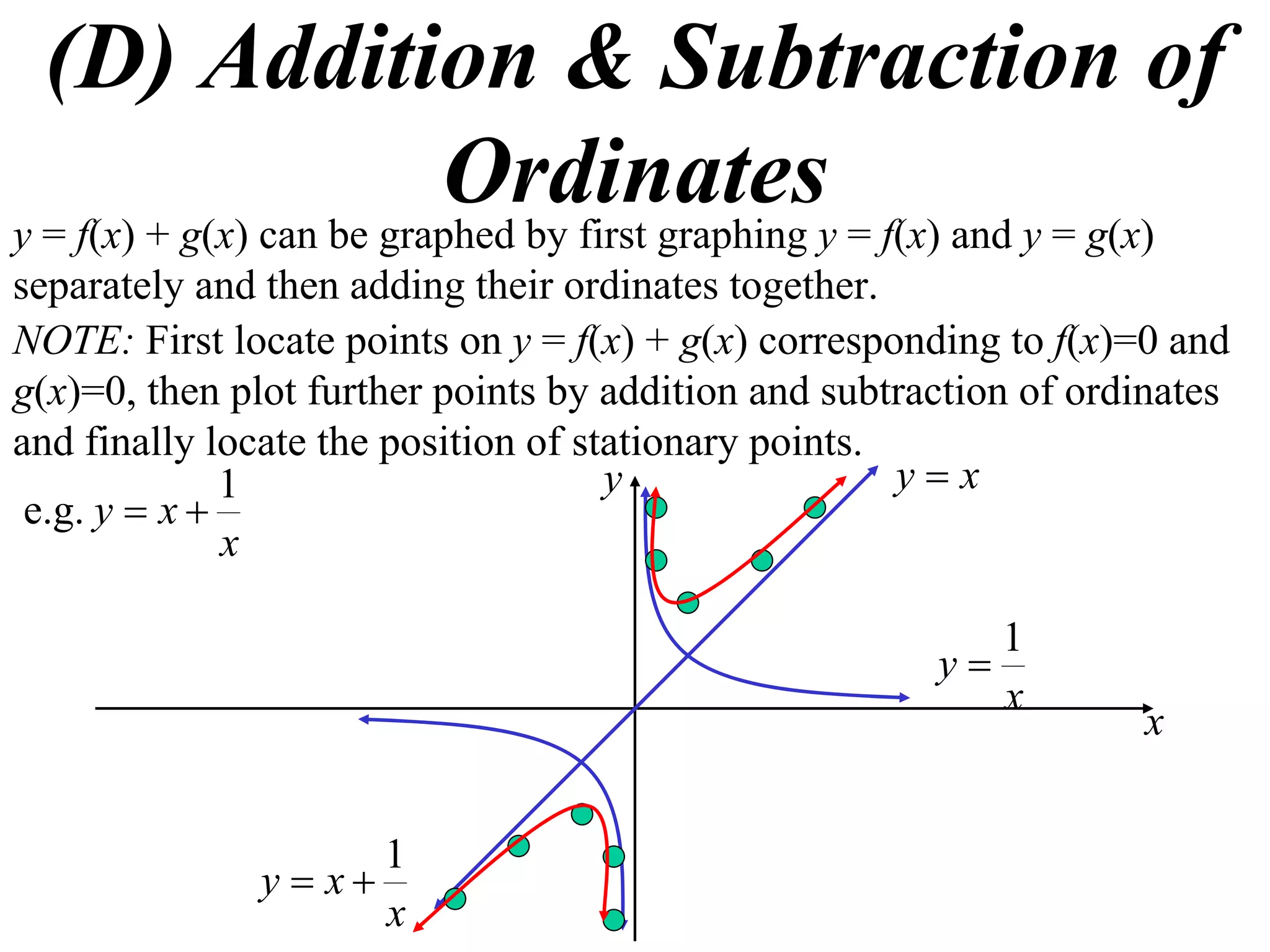
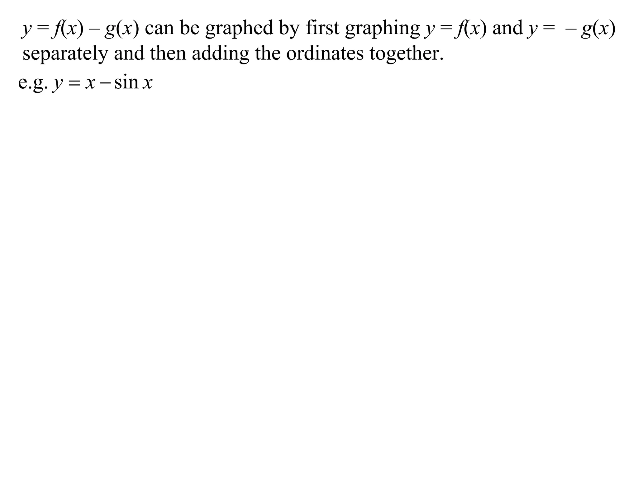
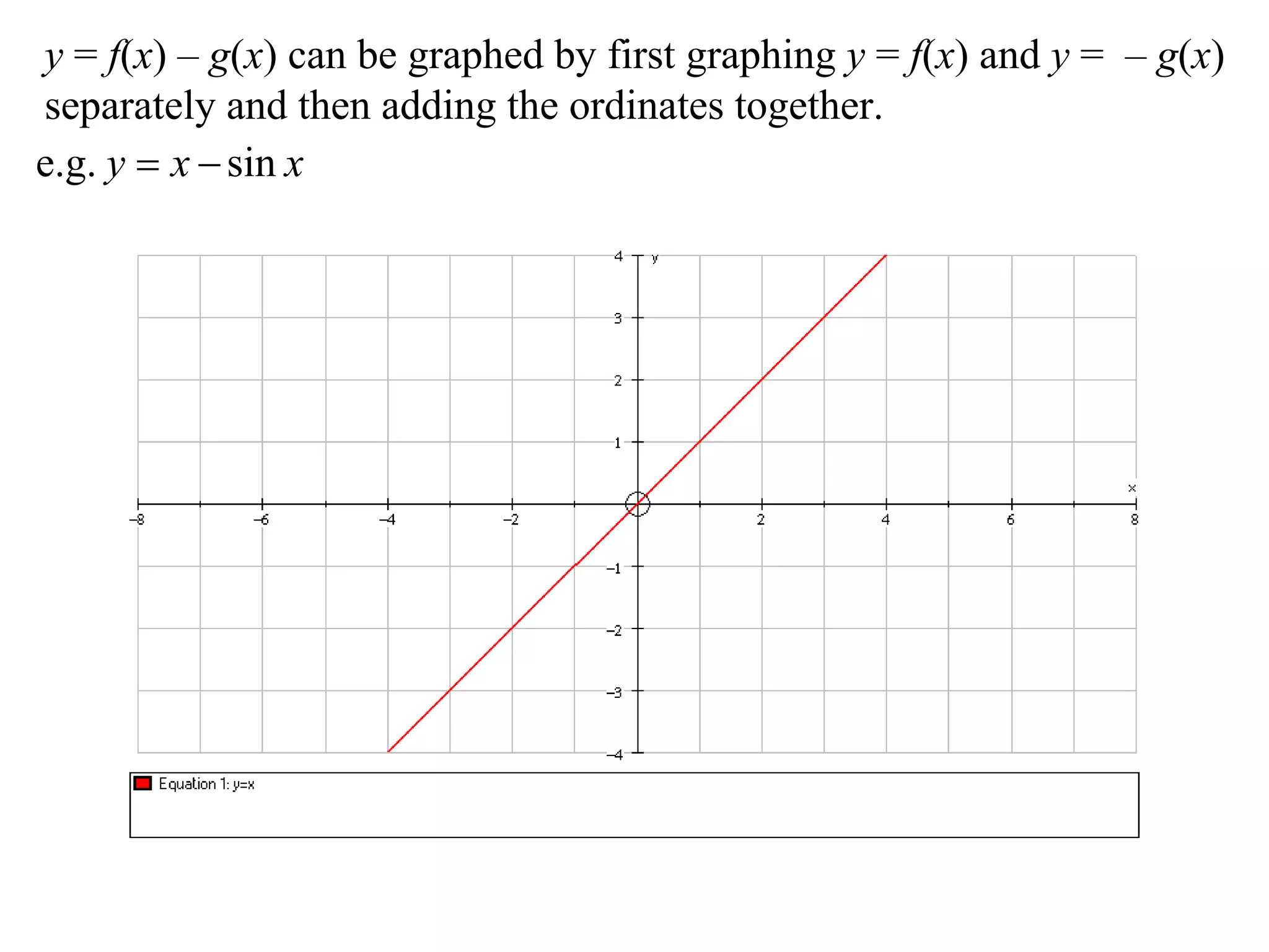
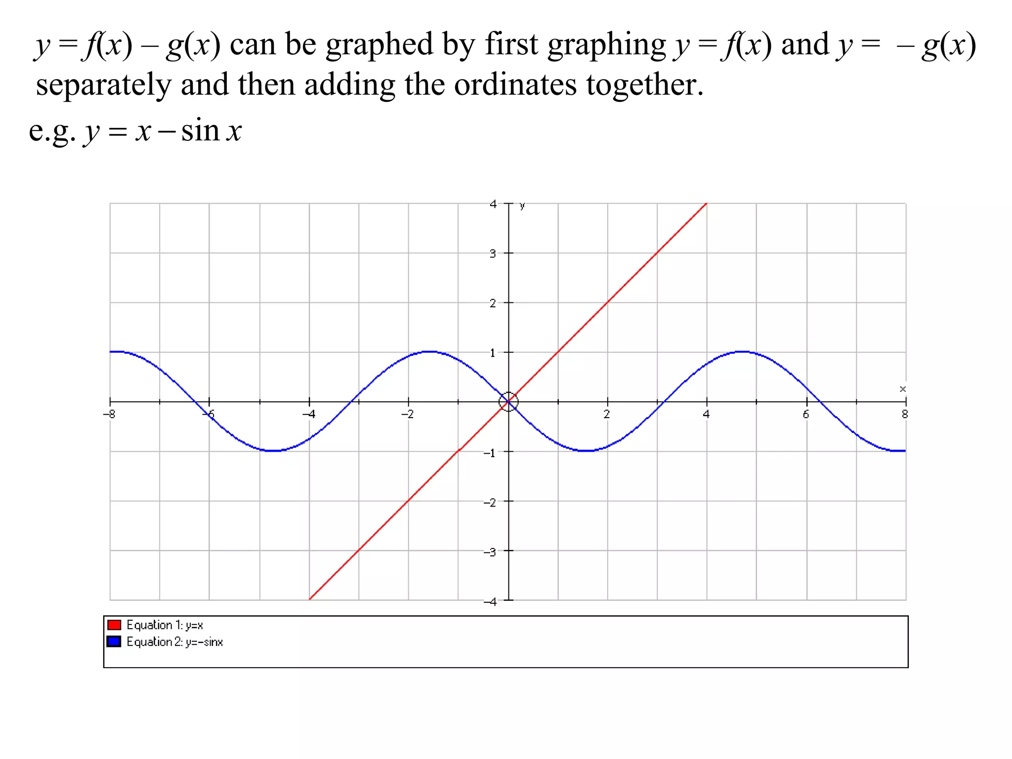
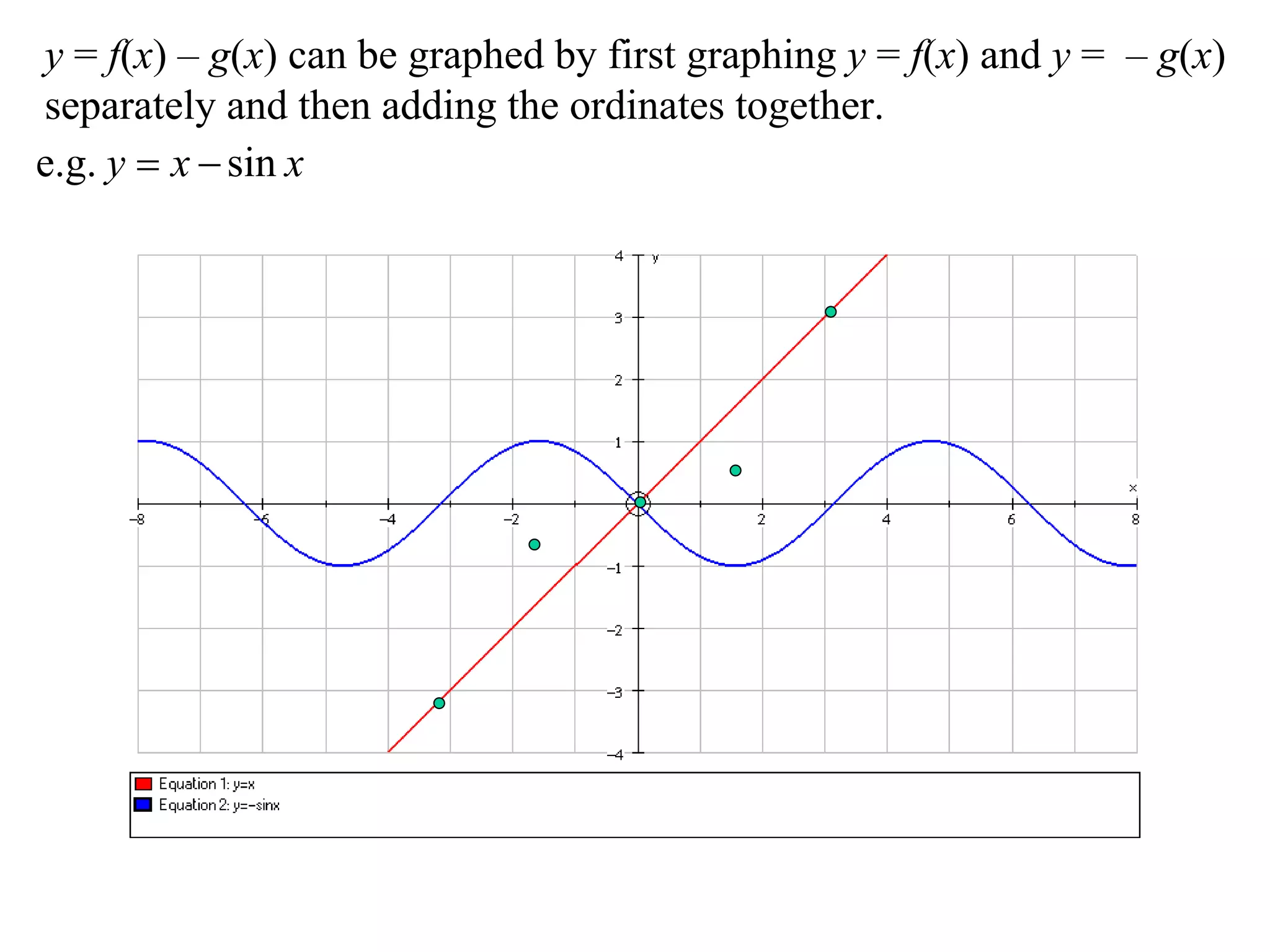
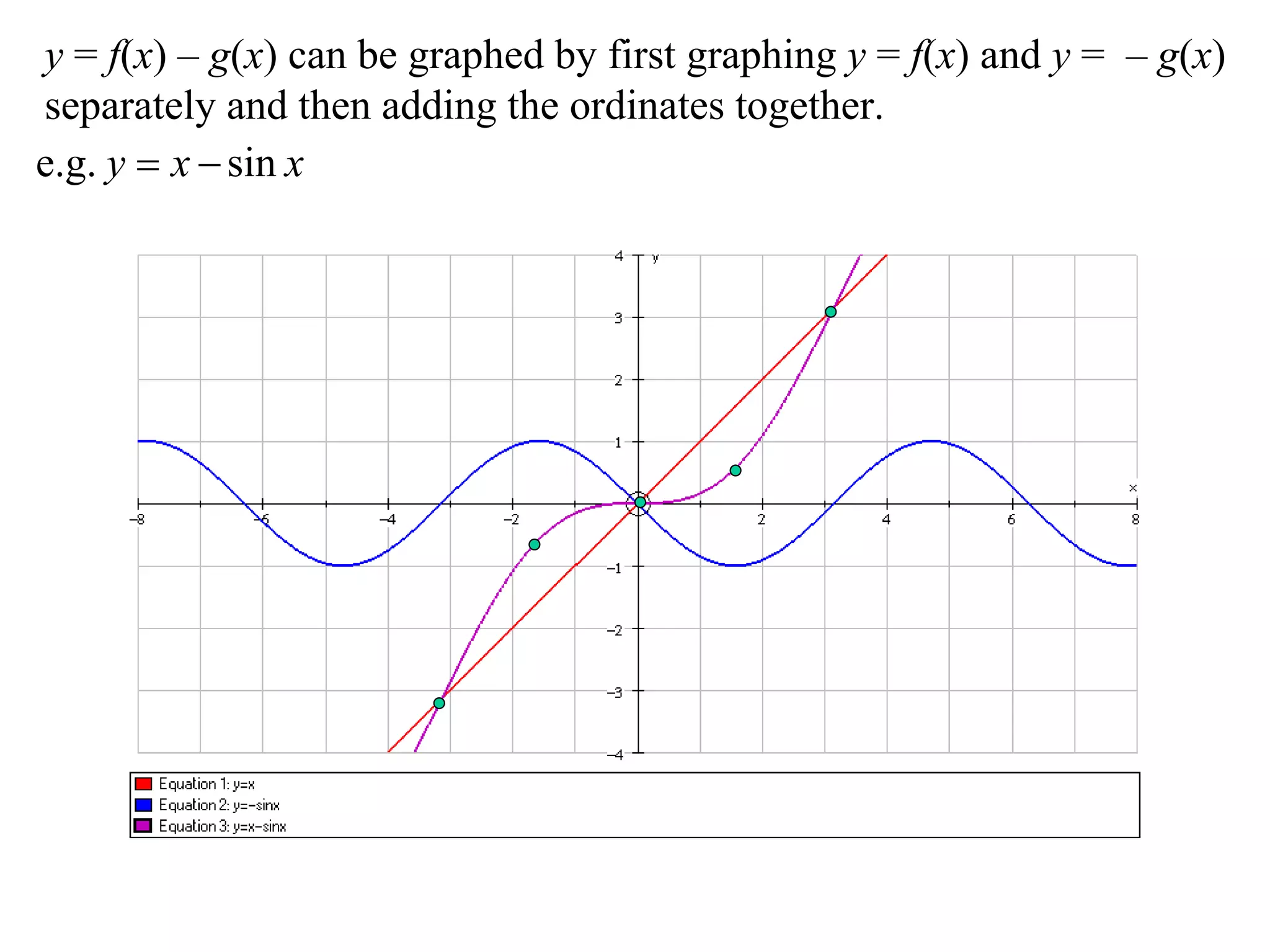
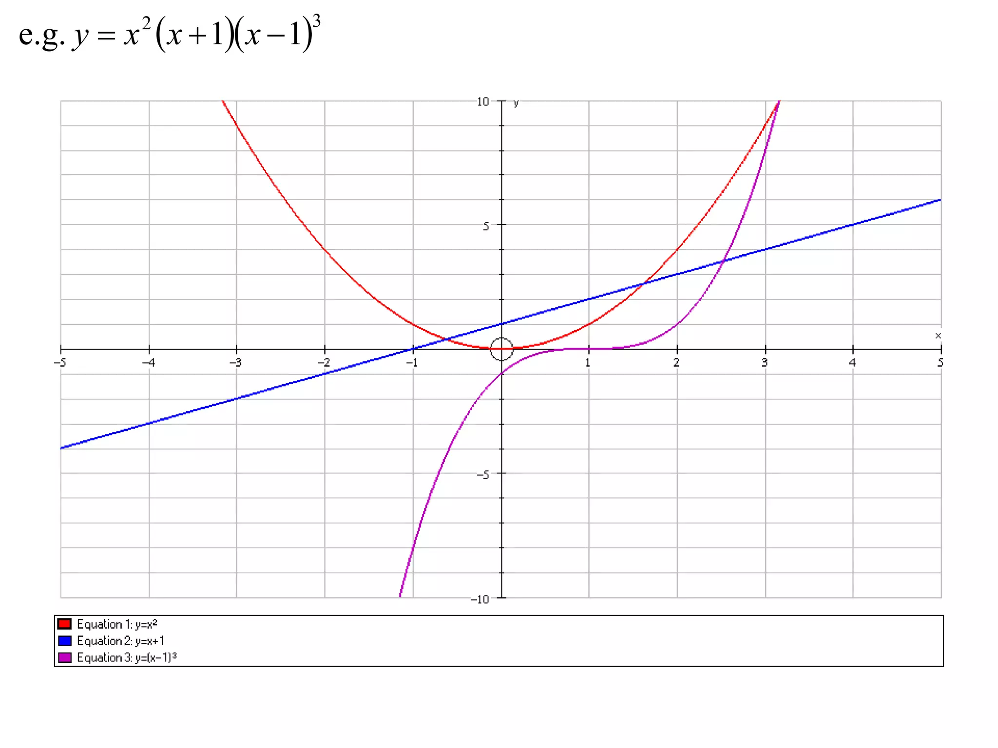
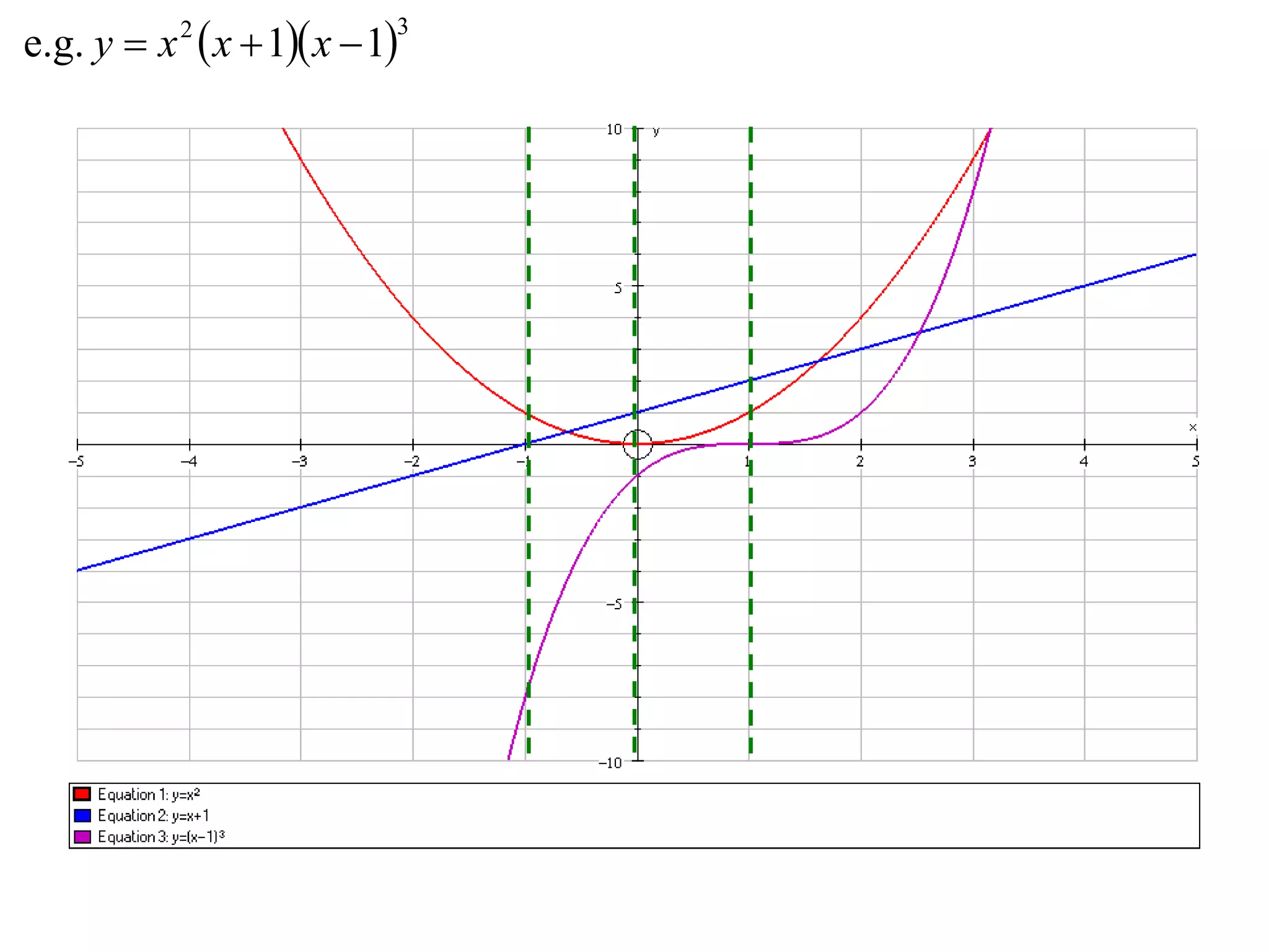
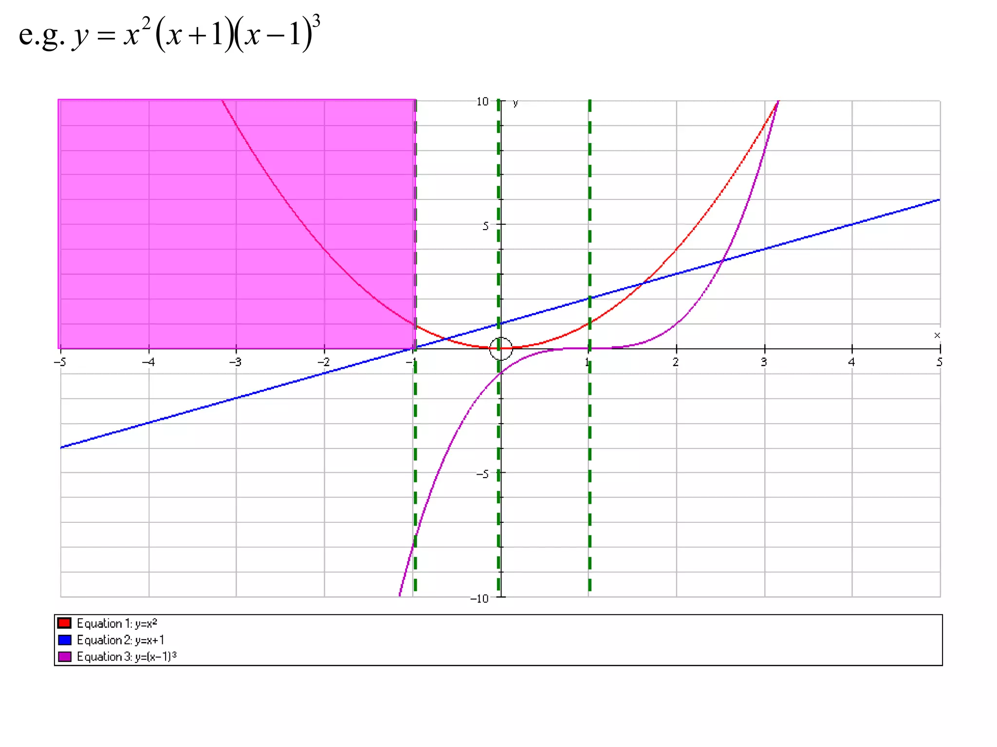
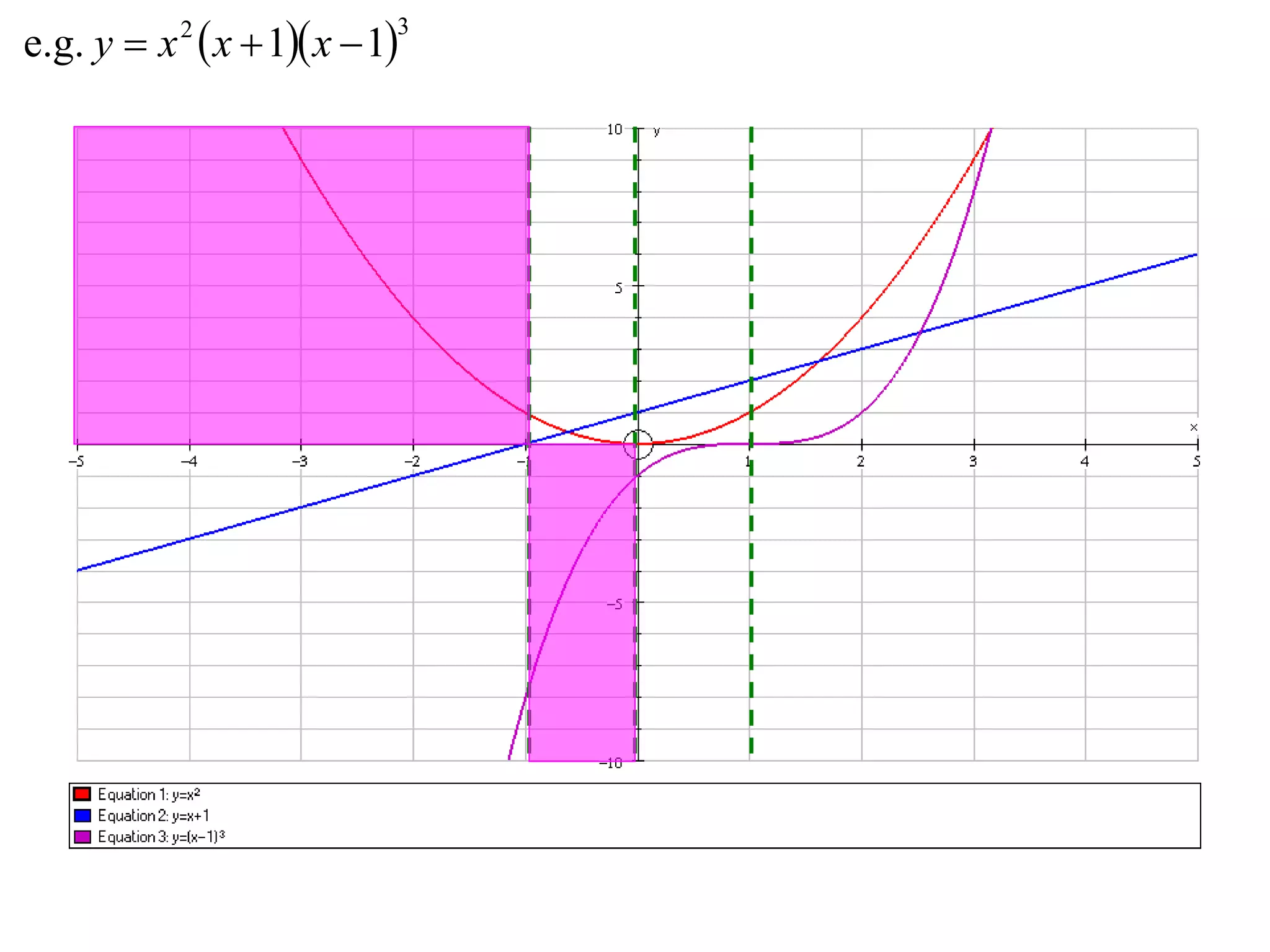
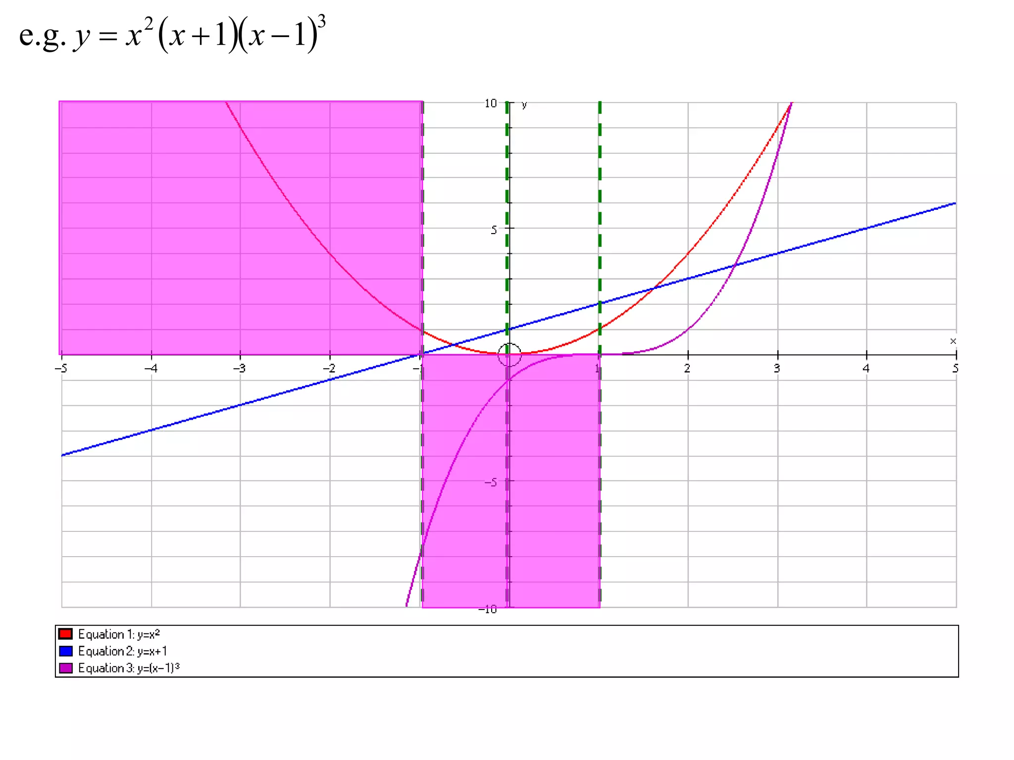
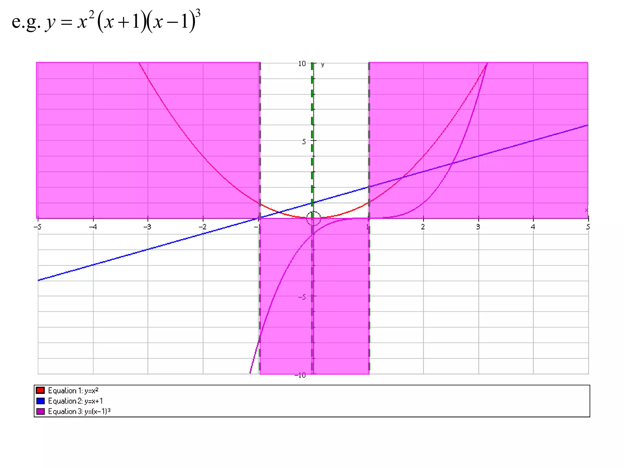
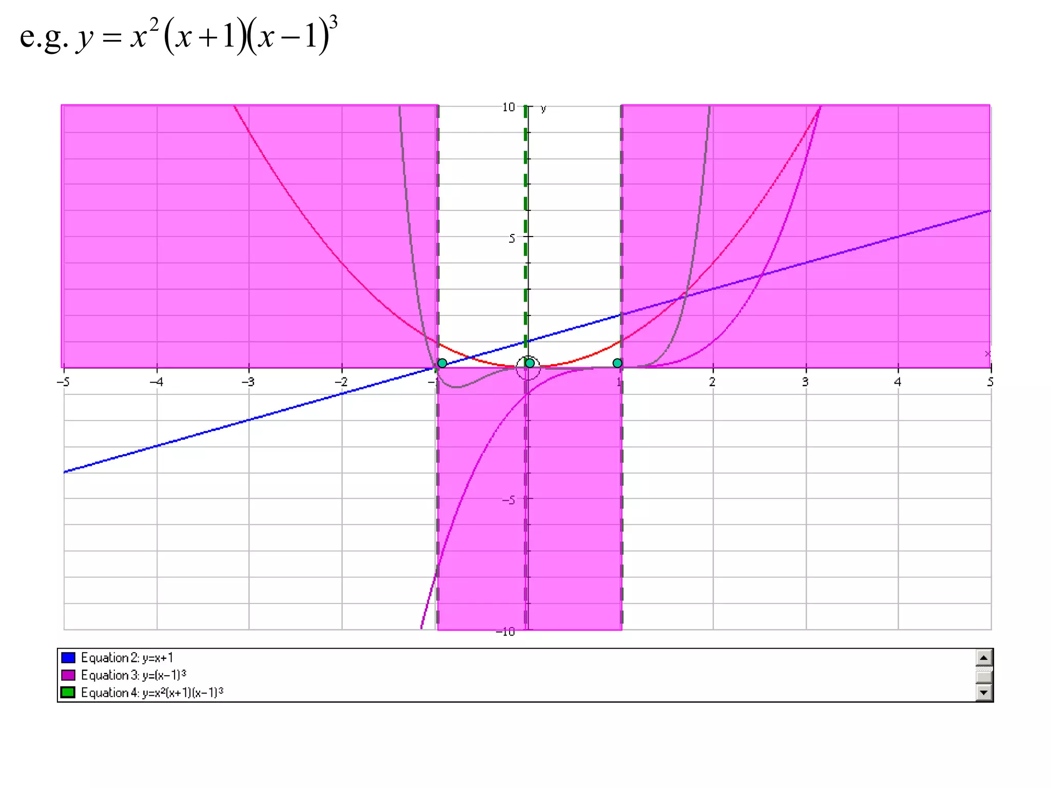
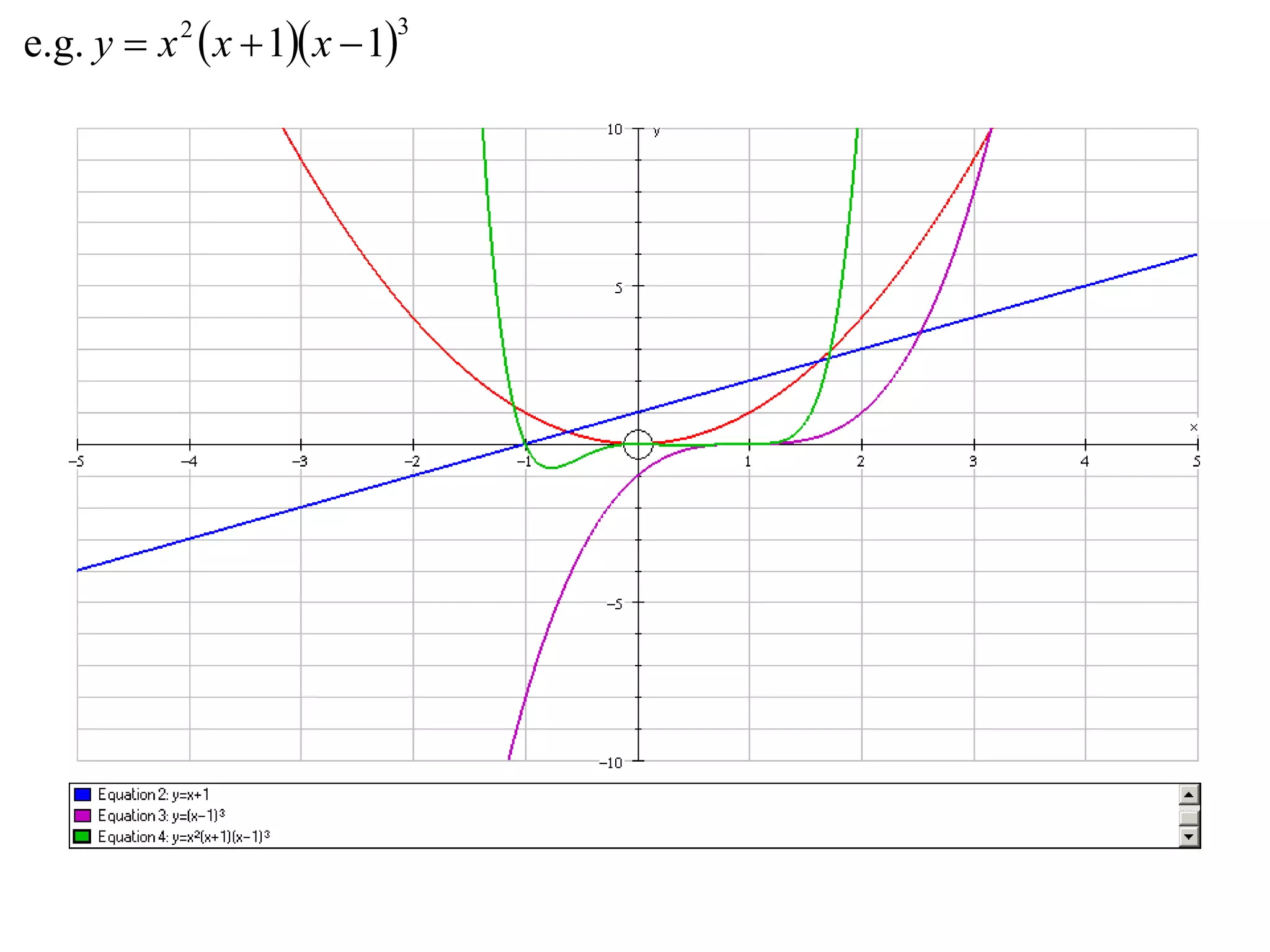
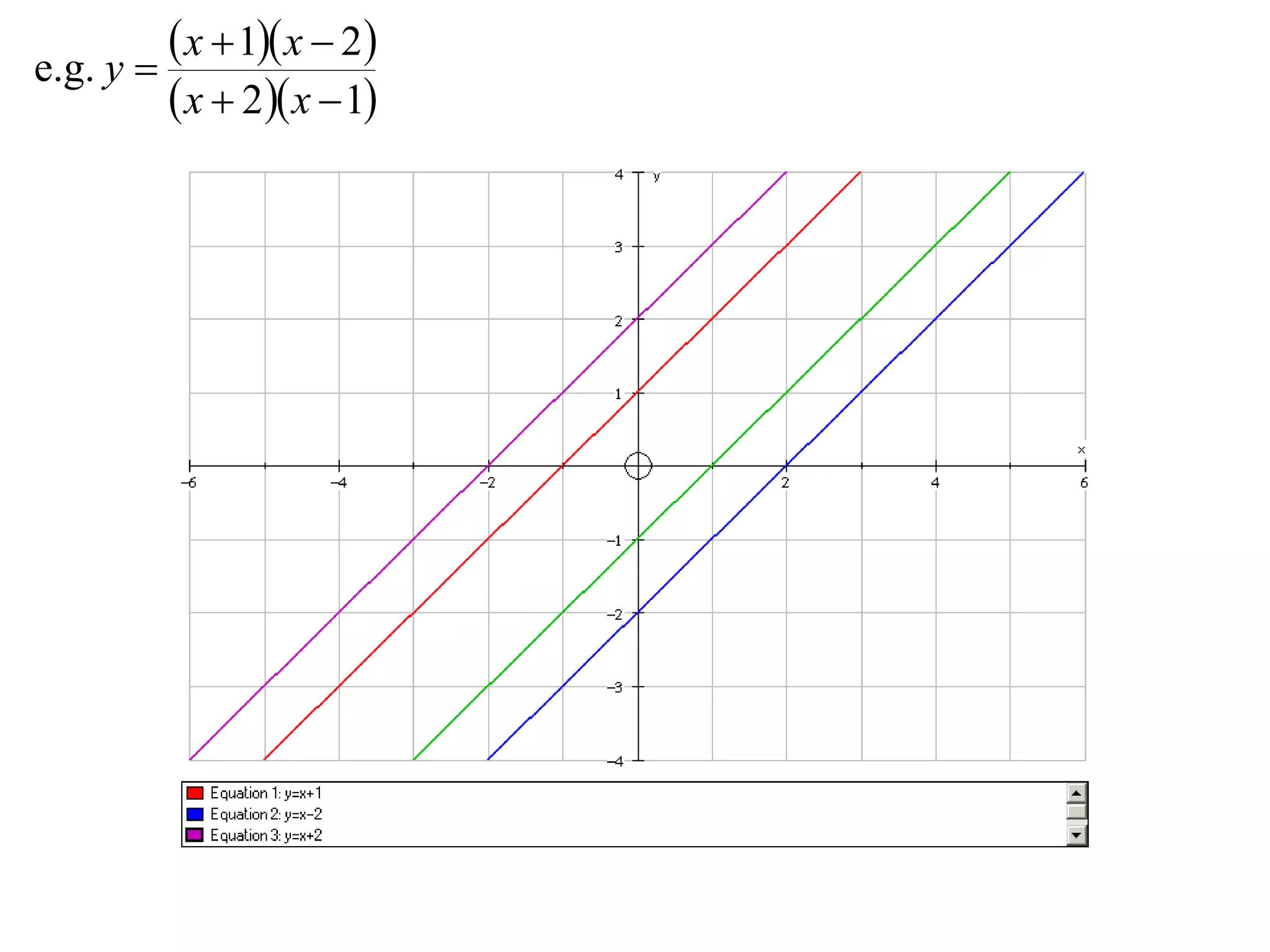
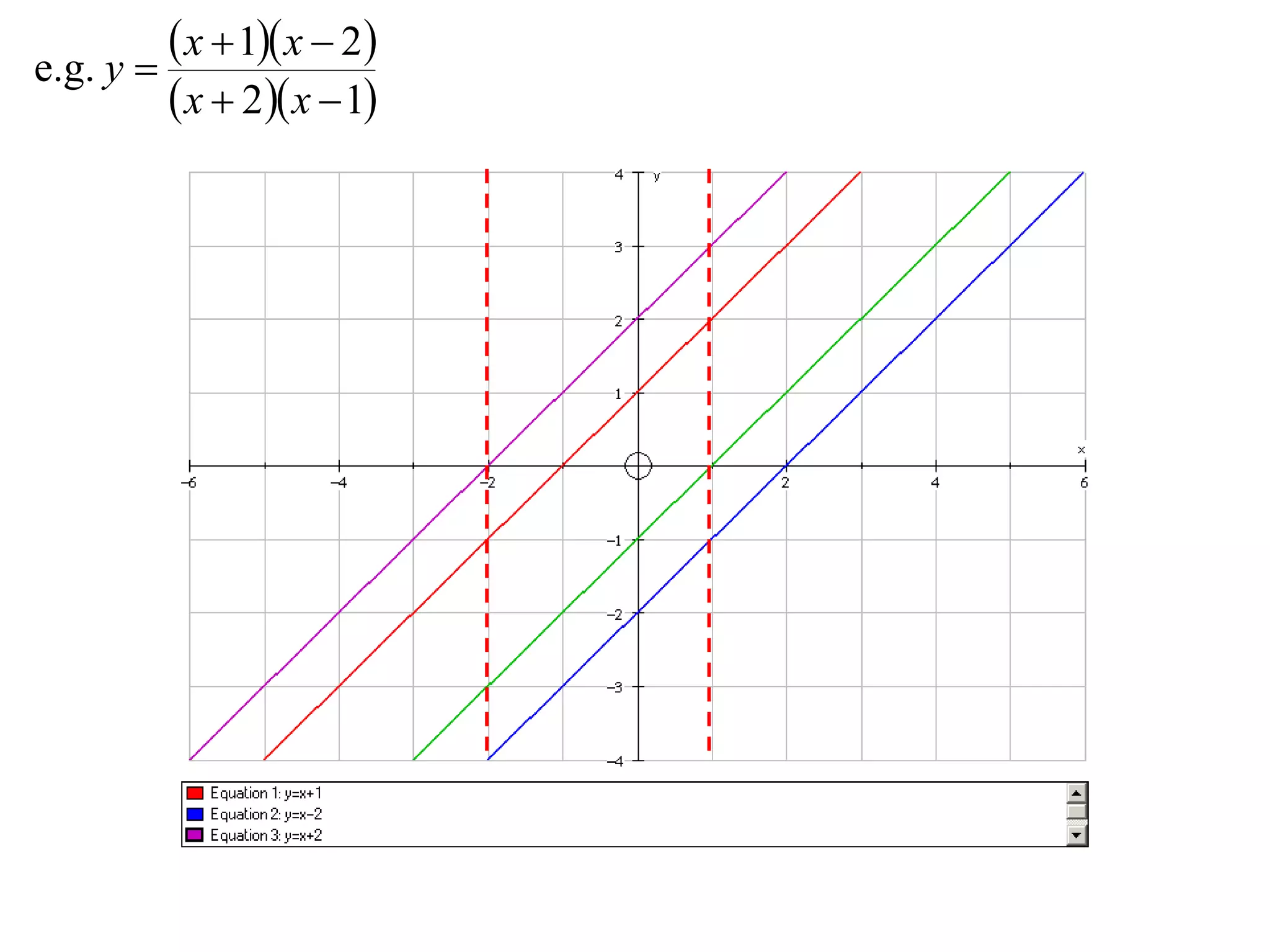
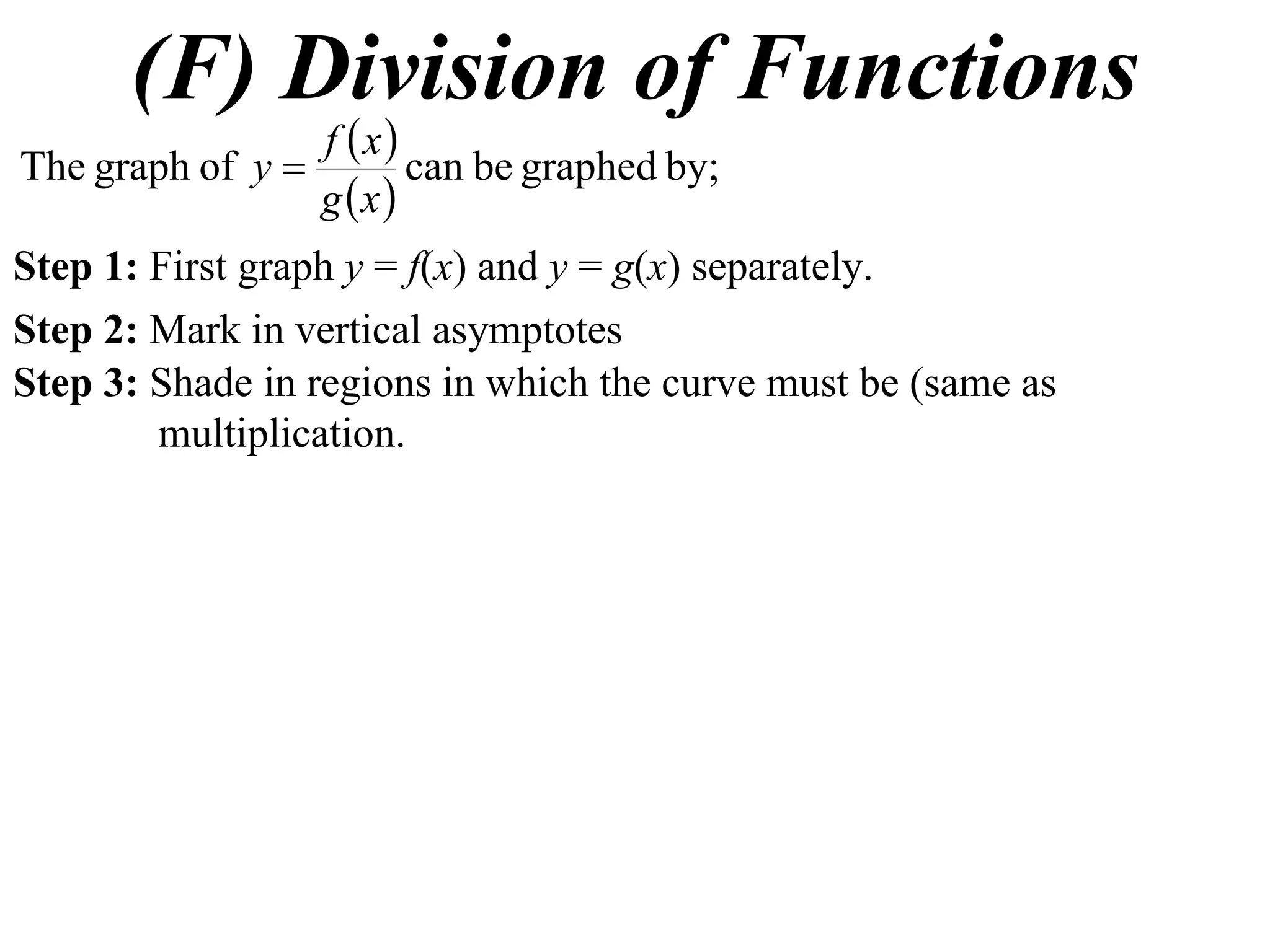
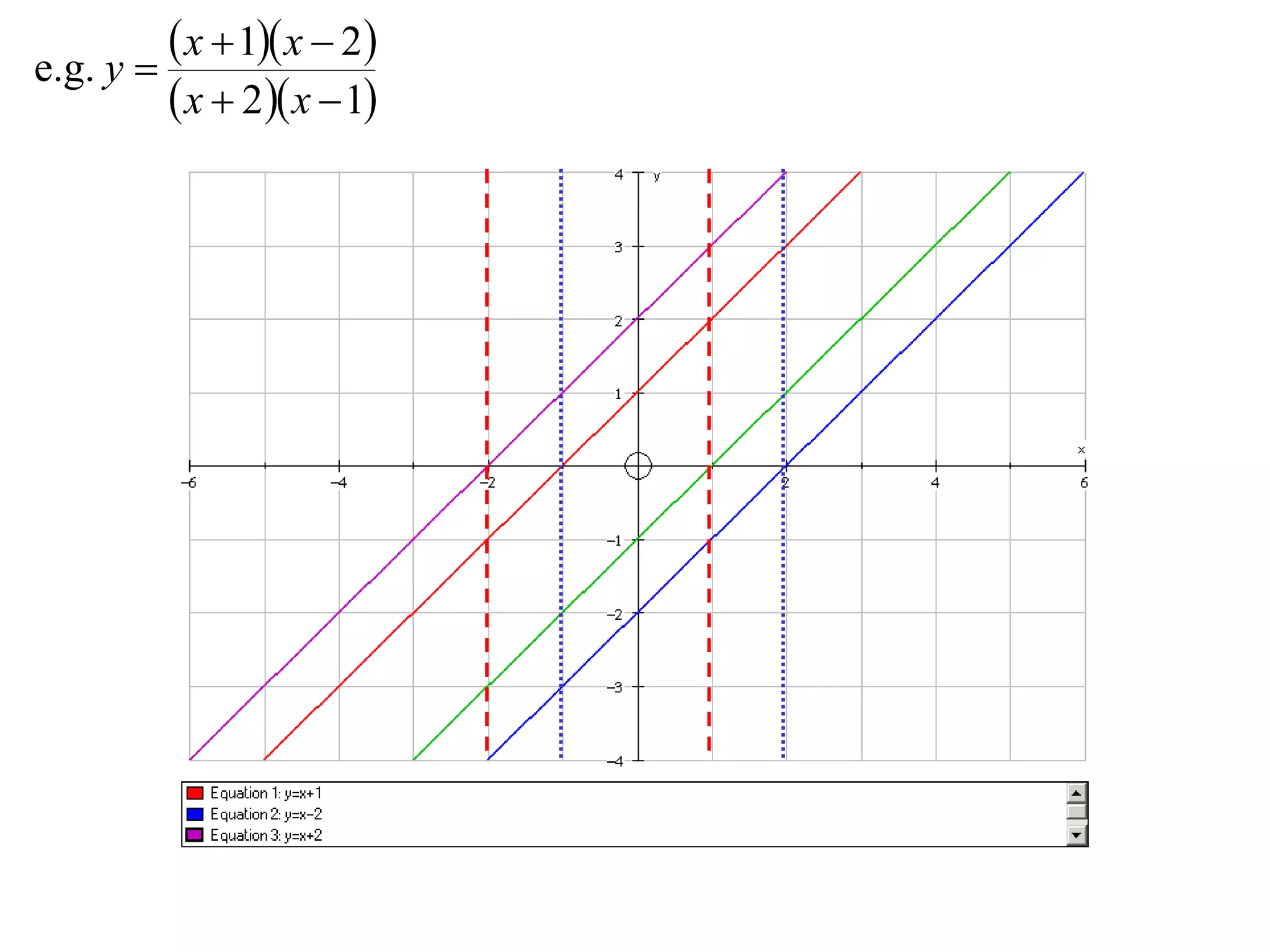
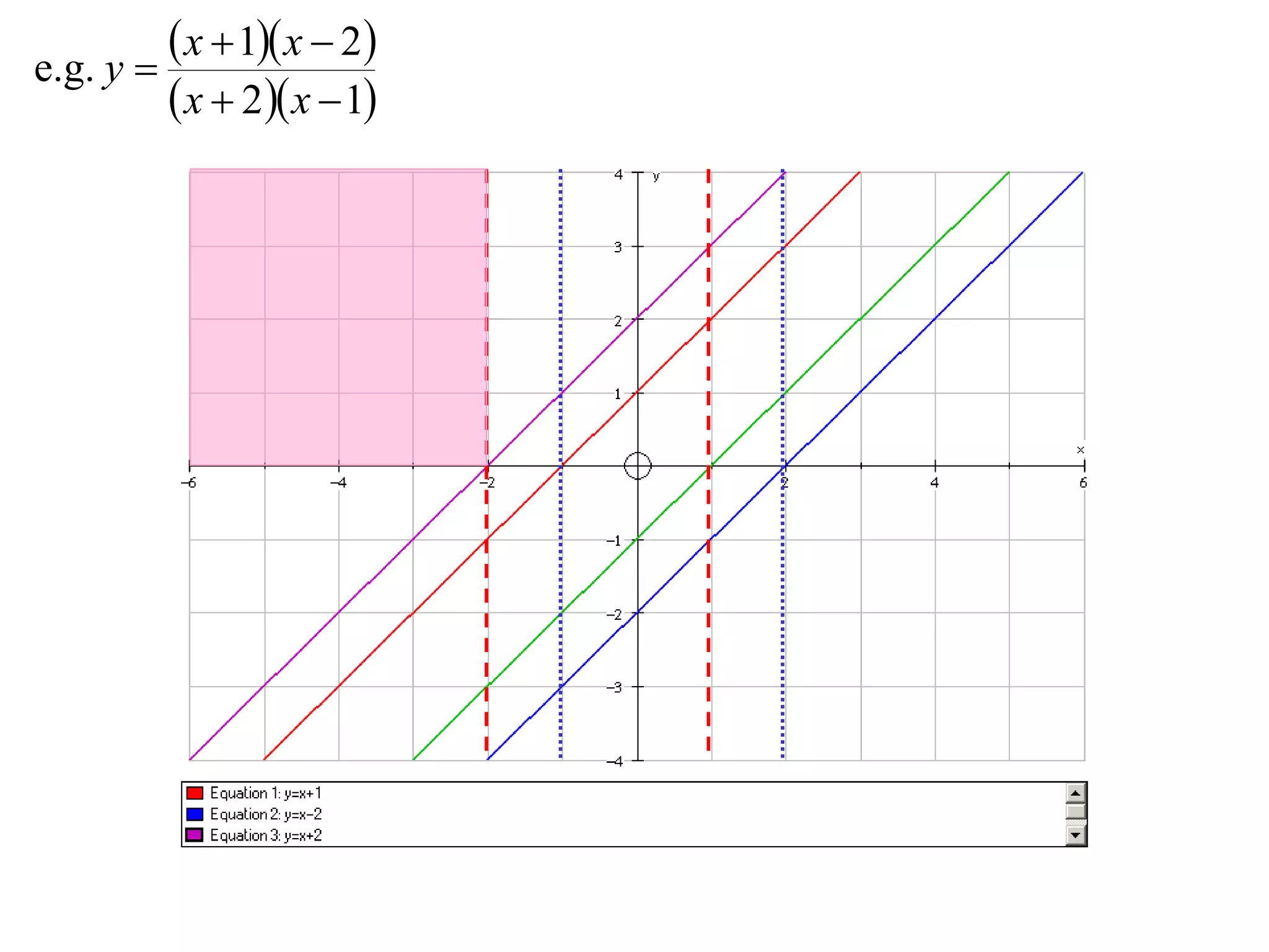
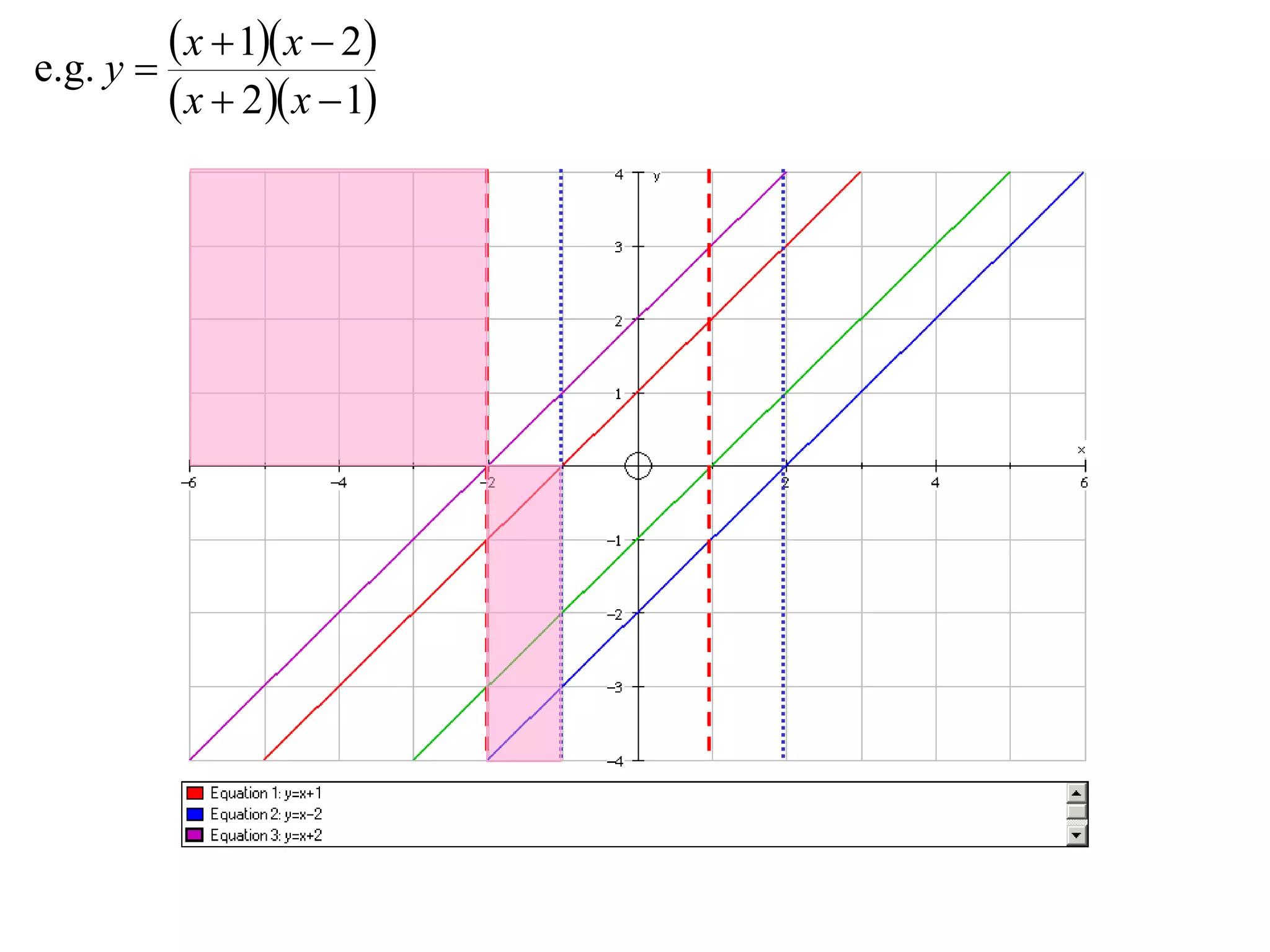
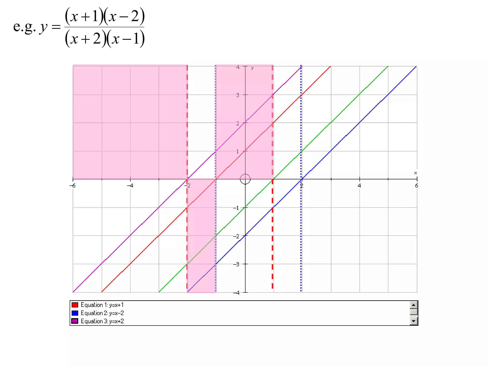
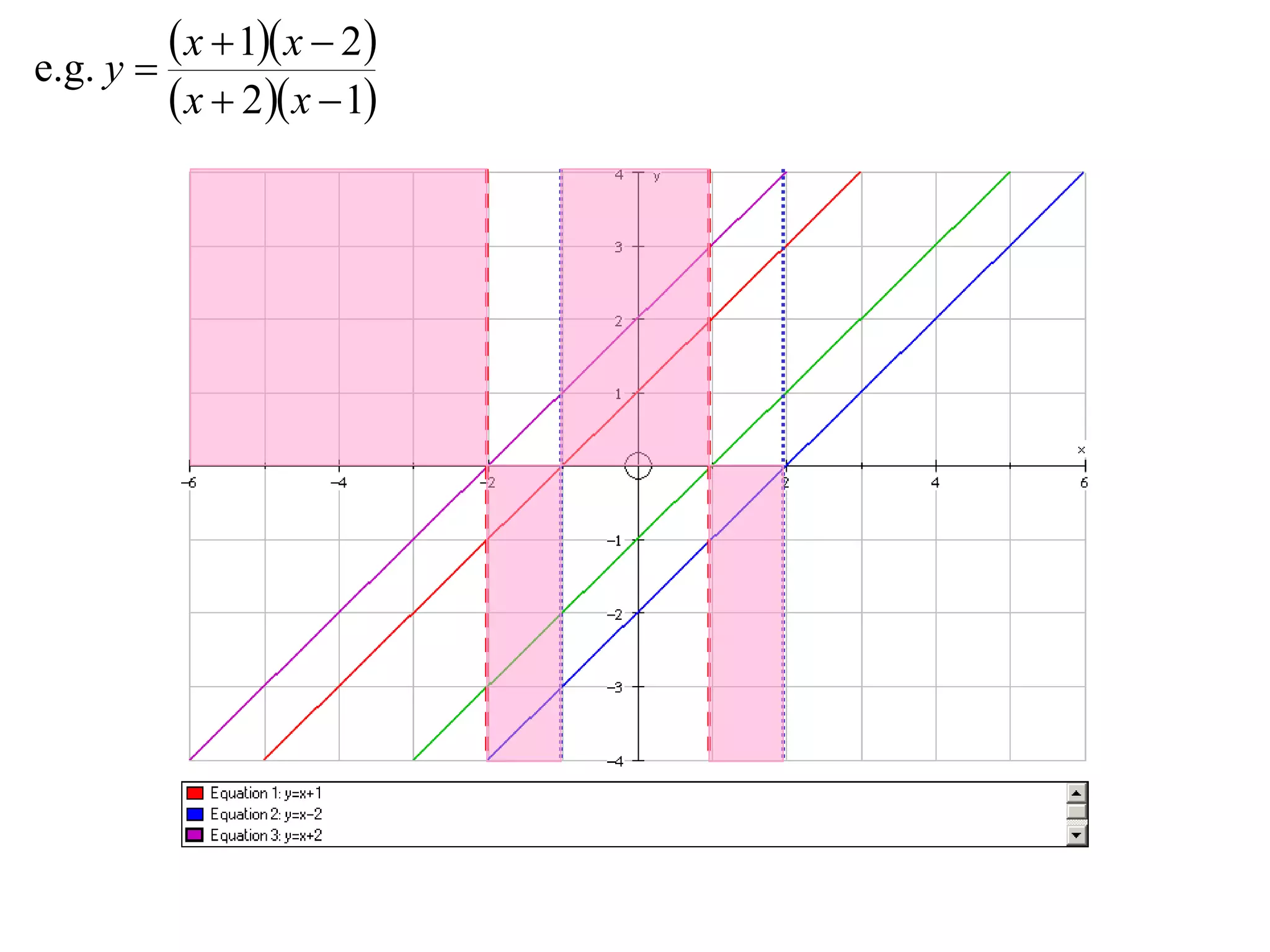
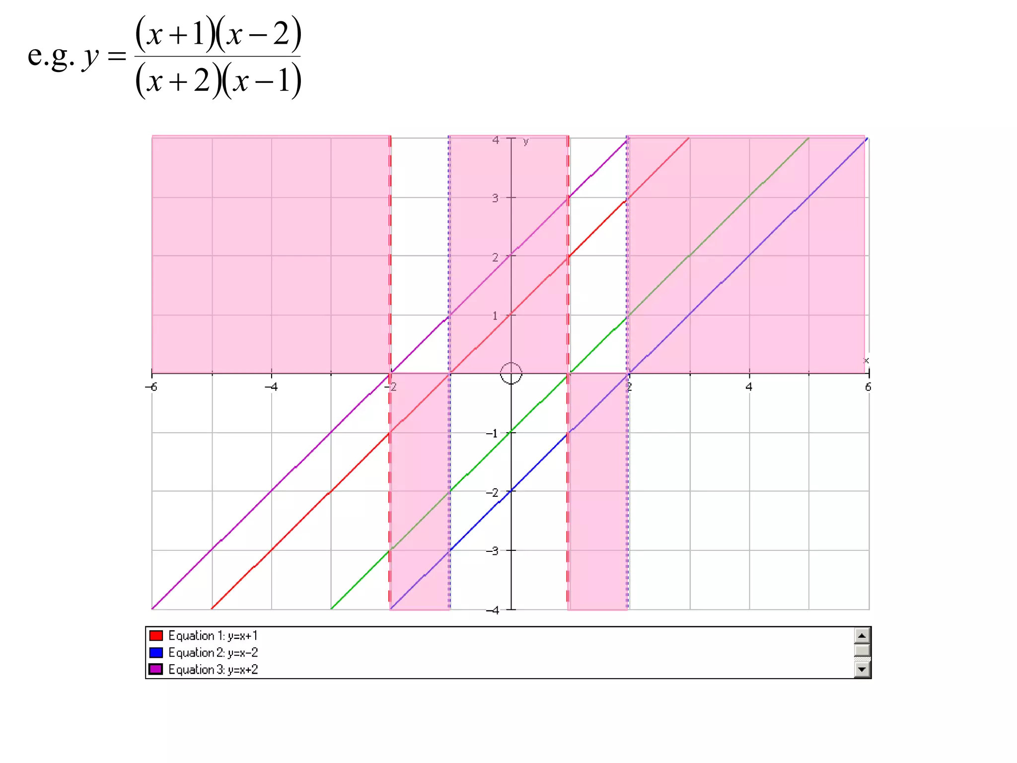
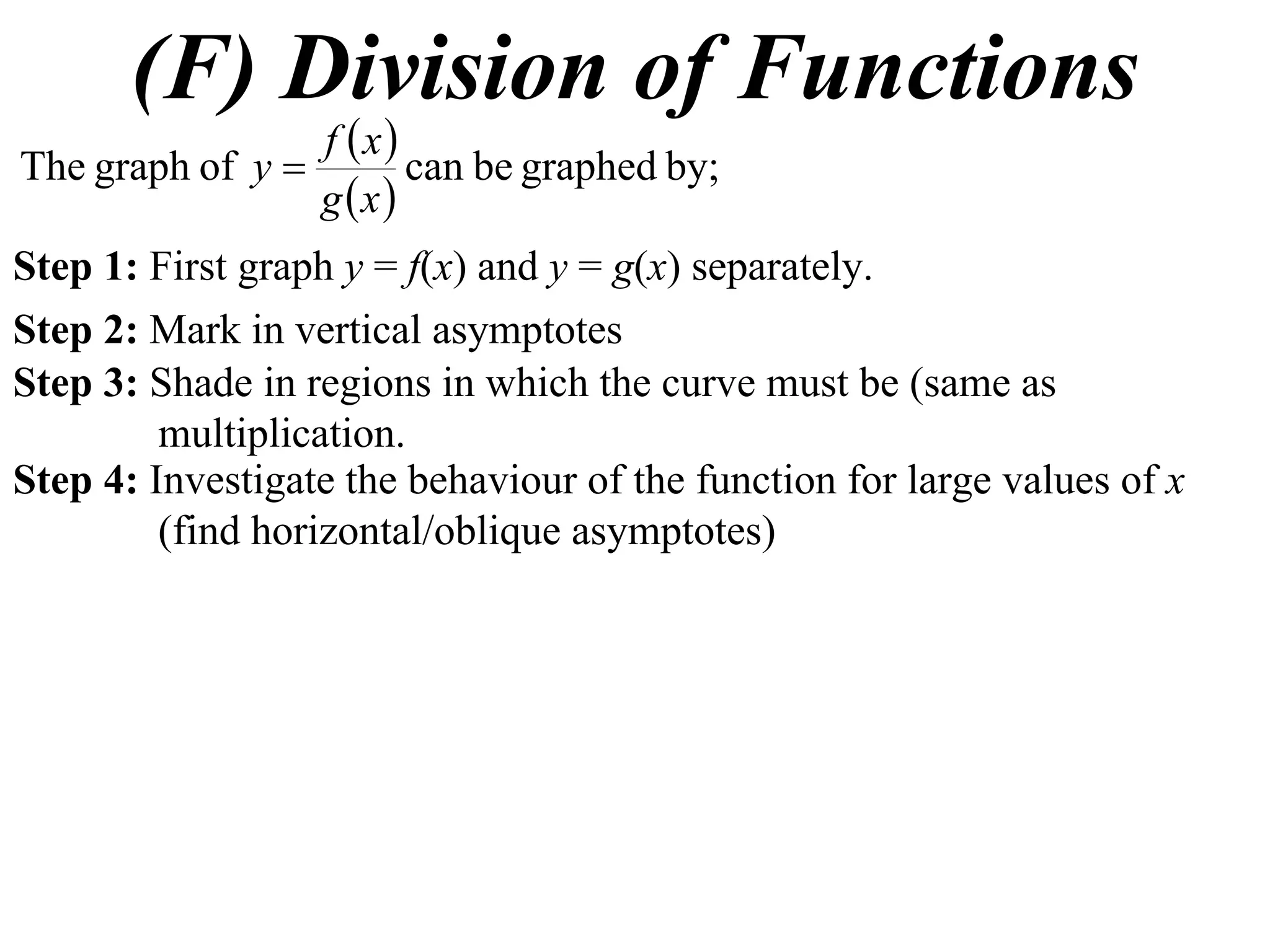
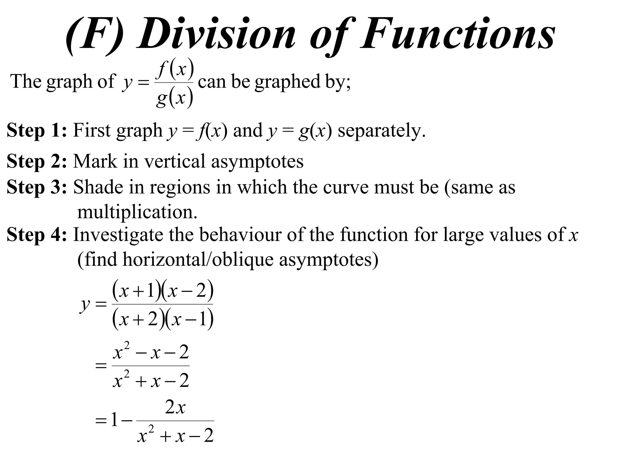
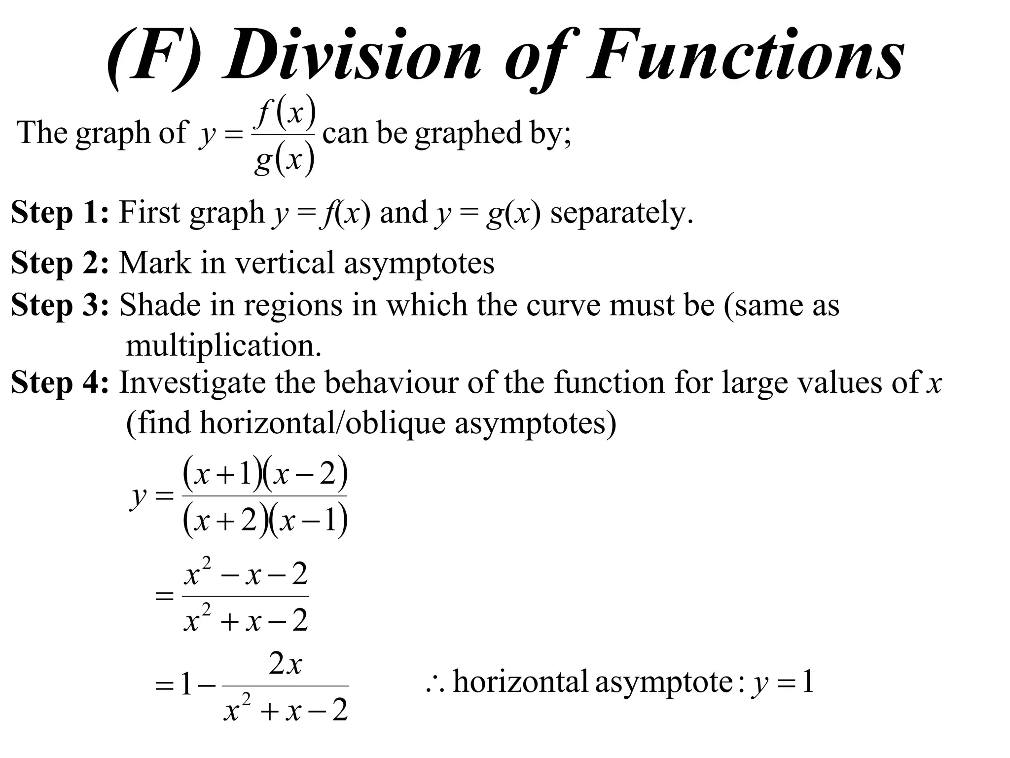
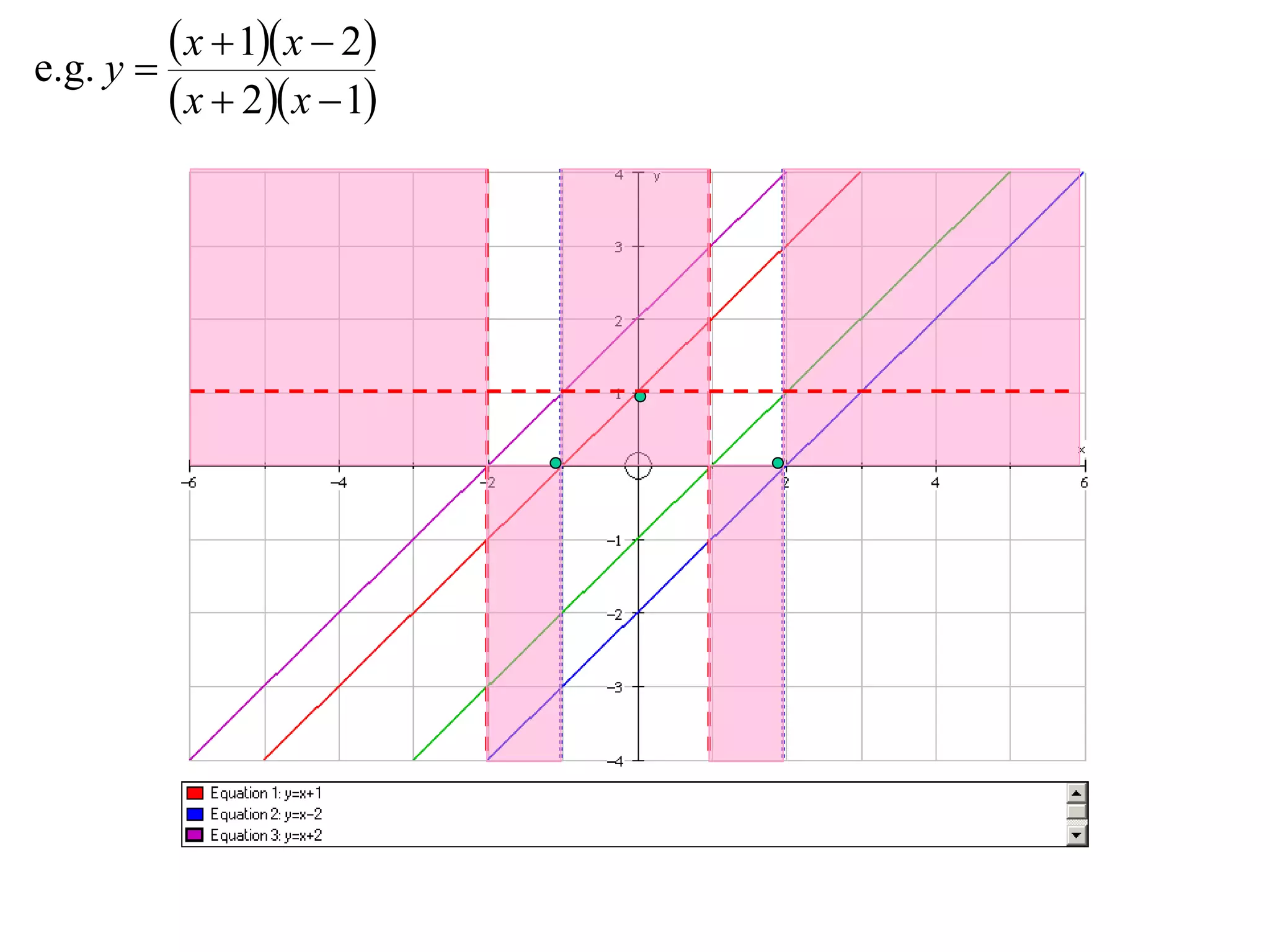
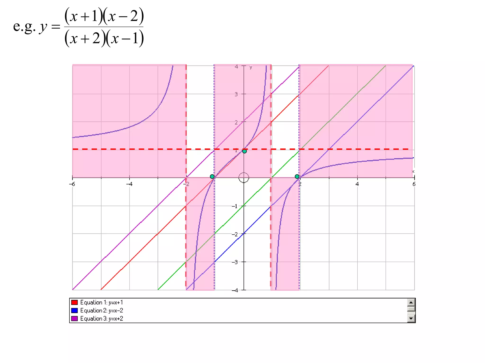
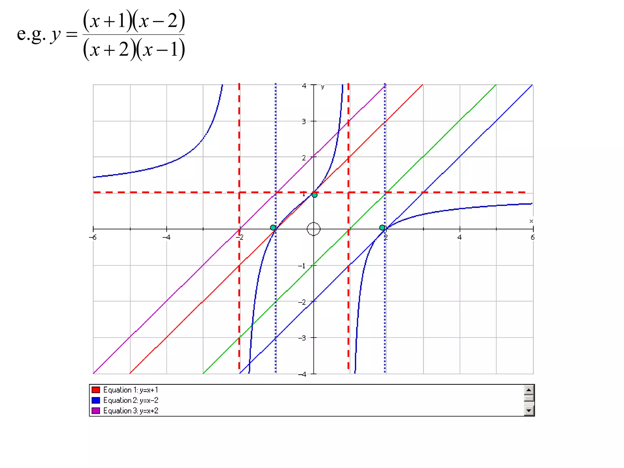
(D) Addition & Subtraction of
          Ordinates
(D) Addition & Subtraction of
                          Ordinatesy = f(x) and y = g(x)
y = f(x) + g(x) can be graphed by first graphing
separately and then adding their ordinates together.
(D) Addition & Subtraction of
                          Ordinatesy = f(x) and y = g(x)
y = f(x) + g(x) can be graphed by first graphing
separately and then adding their ordinates together.
NOTE: First locate points on y = f(x) + g(x) corresponding to f(x)=0 and
g(x)=0, then plot further points by addition and subtraction of ordinates
and finally locate the position of stationary points.
              1
 e.g. y  x 
              x
(D) Addition & Subtraction of
                          Ordinatesy = f(x) and y = g(x)
y = f(x) + g(x) can be graphed by first graphing
separately and then adding their ordinates together.
NOTE: First locate points on y = f(x) + g(x) corresponding to f(x)=0 and
g(x)=0, then plot further points by addition and subtraction of ordinates
and finally locate the position of stationary points.
              1                      y                yx
 e.g. y  x 
              x

                                                            1
                                                       y
                                                            x
                                                                   x


                       1
              y  x
                       x
y = f(x) – g(x) can be graphed by first graphing y = f(x) and y = – g(x)
separately and then adding the ordinates together.
y = f(x) – g(x) can be graphed by first graphing y = f(x) and y = – g(x)
separately and then adding the ordinates together.
e.g. y  x  sin x
y = f(x) – g(x) can be graphed by first graphing y = f(x) and y = – g(x)
separately and then adding the ordinates together.
e.g. y  x  sin x
y = f(x) – g(x) can be graphed by first graphing y = f(x) and y = – g(x)
separately and then adding the ordinates together.
e.g. y  x  sin x
y = f(x) – g(x) can be graphed by first graphing y = f(x) and y = – g(x)
separately and then adding the ordinates together.
e.g. y  x  sin x
y = f(x) – g(x) can be graphed by first graphing y = f(x) and y = – g(x)
separately and then adding the ordinates together.
e.g. y  x  sin x
y = f(x) – g(x) can be graphed by first graphing y = f(x) and y = – g(x)
separately and then adding the ordinates together.
e.g. y  x  sin x
(E) Multiplication of Functions
The graph of y = f(x). g(x) can be graphed by first graphing y = f(x) and
y= g(x) separately and then examining the sign of the product. Special
note needs to be made of points where f(x) = 0 or 1, or g(x) = 0 or 1.
NOTE: The regions on the number plane through which the graph must
pass should be shaded in as the first step.
e.g. y  x 2  x  1 x  1
                            3
e.g. y  x 2  x  1 x  1
                            3
e.g. y  x 2  x  1 x  1
                            3
e.g. y  x 2  x  1 x  1
                            3
e.g. y  x 2  x  1 x  1
                            3
e.g. y  x 2  x  1 x  1
                            3
e.g. y  x 2  x  1 x  1
                            3
e.g. y  x 2  x  1 x  1
                            3
e.g. y  x 2  x  1 x  1
                            3
(F) Division of Functions
                 f x
The graph of y        can be graphed by;
                 g x
(F) Division of Functions
                 f x
The graph of y        can be graphed by;
                 g x
Step 1: First graph y = f(x) and y = g(x) separately.
e.g. y 
          x  1 x  2
          x  2 x  1
e.g. y 
          x  1 x  2
          x  2 x  1
(F) Division of Functions
                 f x
The graph of y        can be graphed by;
                 g x
Step 1: First graph y = f(x) and y = g(x) separately.
Step 2: Mark in vertical asymptotes
e.g. y 
          x  1 x  2
          x  2 x  1
(F) Division of Functions
                 f x
The graph of y        can be graphed by;
                 g x
Step 1: First graph y = f(x) and y = g(x) separately.
Step 2: Mark in vertical asymptotes
Step 3: Shade in regions in which the curve must be (same as
        multiplication.
e.g. y 
          x  1 x  2
          x  2 x  1
e.g. y 
          x  1 x  2
          x  2 x  1
e.g. y 
          x  1 x  2
          x  2 x  1
e.g. y 
          x  1 x  2
          x  2 x  1
e.g. y 
          x  1 x  2
          x  2 x  1
e.g. y 
          x  1 x  2
          x  2 x  1
e.g. y 
          x  1 x  2
          x  2 x  1
(F) Division of Functions
                 f x
The graph of y        can be graphed by;
                 g x
Step 1: First graph y = f(x) and y = g(x) separately.
Step 2: Mark in vertical asymptotes
Step 3: Shade in regions in which the curve must be (same as
         multiplication.
Step 4: Investigate the behaviour of the function for large values of x
         (find horizontal/oblique asymptotes)
              x  1 x  2
          y
              x  2 x  1
             x2  x  2
            2
             x  x2
                    2x
            1 2
                x  x2
(F) Division of Functions
                 f x
The graph of y        can be graphed by;
                 g x
Step 1: First graph y = f(x) and y = g(x) separately.
Step 2: Mark in vertical asymptotes
Step 3: Shade in regions in which the curve must be (same as
         multiplication.
Step 4: Investigate the behaviour of the function for large values of x
         (find horizontal/oblique asymptotes)
              x  1 x  2
          y
              x  2 x  1
             x2  x  2
            2
             x  x2
                    2x
            1 2               horizontal asymptote : y  1
                x  x2
e.g. y 
          x  1 x  2
          x  2 x  1
e.g. y 
          x  1 x  2
          x  2 x  1
e.g. y 
          x  1 x  2
          x  2 x  1

X2 T07 03 addition, subtraction, multiplication & division (2011)

  • 1.
    (D) Addition &Subtraction of Ordinates
  • 2.
    (D) Addition &Subtraction of Ordinatesy = f(x) and y = g(x) y = f(x) + g(x) can be graphed by first graphing separately and then adding their ordinates together.
  • 3.
    (D) Addition &Subtraction of Ordinatesy = f(x) and y = g(x) y = f(x) + g(x) can be graphed by first graphing separately and then adding their ordinates together. NOTE: First locate points on y = f(x) + g(x) corresponding to f(x)=0 and g(x)=0, then plot further points by addition and subtraction of ordinates and finally locate the position of stationary points.
  • 4.
    (D) Addition &Subtraction of Ordinatesy = f(x) and y = g(x) y = f(x) + g(x) can be graphed by first graphing separately and then adding their ordinates together. NOTE: First locate points on y = f(x) + g(x) corresponding to f(x)=0 and g(x)=0, then plot further points by addition and subtraction of ordinates and finally locate the position of stationary points. 1 e.g. y  x  x
  • 5.
    (D) Addition &Subtraction of Ordinatesy = f(x) and y = g(x) y = f(x) + g(x) can be graphed by first graphing separately and then adding their ordinates together. NOTE: First locate points on y = f(x) + g(x) corresponding to f(x)=0 and g(x)=0, then plot further points by addition and subtraction of ordinates and finally locate the position of stationary points. 1 y yx e.g. y  x  x 1 y x x
  • 6.
    (D) Addition &Subtraction of Ordinatesy = f(x) and y = g(x) y = f(x) + g(x) can be graphed by first graphing separately and then adding their ordinates together. NOTE: First locate points on y = f(x) + g(x) corresponding to f(x)=0 and g(x)=0, then plot further points by addition and subtraction of ordinates and finally locate the position of stationary points. 1 y yx e.g. y  x  x 1 y x x
  • 7.
    (D) Addition &Subtraction of Ordinatesy = f(x) and y = g(x) y = f(x) + g(x) can be graphed by first graphing separately and then adding their ordinates together. NOTE: First locate points on y = f(x) + g(x) corresponding to f(x)=0 and g(x)=0, then plot further points by addition and subtraction of ordinates and finally locate the position of stationary points. 1 y yx e.g. y  x  x 1 y x x 1 y  x x
  • 8.
    y = f(x)– g(x) can be graphed by first graphing y = f(x) and y = – g(x) separately and then adding the ordinates together.
  • 9.
    y = f(x)– g(x) can be graphed by first graphing y = f(x) and y = – g(x) separately and then adding the ordinates together. e.g. y  x  sin x
  • 10.
    y = f(x)– g(x) can be graphed by first graphing y = f(x) and y = – g(x) separately and then adding the ordinates together. e.g. y  x  sin x
  • 11.
    y = f(x)– g(x) can be graphed by first graphing y = f(x) and y = – g(x) separately and then adding the ordinates together. e.g. y  x  sin x
  • 12.
    y = f(x)– g(x) can be graphed by first graphing y = f(x) and y = – g(x) separately and then adding the ordinates together. e.g. y  x  sin x
  • 13.
    y = f(x)– g(x) can be graphed by first graphing y = f(x) and y = – g(x) separately and then adding the ordinates together. e.g. y  x  sin x
  • 14.
    y = f(x)– g(x) can be graphed by first graphing y = f(x) and y = – g(x) separately and then adding the ordinates together. e.g. y  x  sin x
  • 15.
    (E) Multiplication ofFunctions The graph of y = f(x). g(x) can be graphed by first graphing y = f(x) and y= g(x) separately and then examining the sign of the product. Special note needs to be made of points where f(x) = 0 or 1, or g(x) = 0 or 1. NOTE: The regions on the number plane through which the graph must pass should be shaded in as the first step.
  • 16.
    e.g. y x 2  x  1 x  1 3
  • 17.
    e.g. y x 2  x  1 x  1 3
  • 18.
    e.g. y x 2  x  1 x  1 3
  • 19.
    e.g. y x 2  x  1 x  1 3
  • 20.
    e.g. y x 2  x  1 x  1 3
  • 21.
    e.g. y x 2  x  1 x  1 3
  • 22.
    e.g. y x 2  x  1 x  1 3
  • 23.
    e.g. y x 2  x  1 x  1 3
  • 24.
    e.g. y x 2  x  1 x  1 3
  • 25.
    (F) Division ofFunctions f x The graph of y  can be graphed by; g x
  • 26.
    (F) Division ofFunctions f x The graph of y  can be graphed by; g x Step 1: First graph y = f(x) and y = g(x) separately.
  • 27.
    e.g. y   x  1 x  2  x  2 x  1
  • 28.
    e.g. y   x  1 x  2  x  2 x  1
  • 29.
    (F) Division ofFunctions f x The graph of y  can be graphed by; g x Step 1: First graph y = f(x) and y = g(x) separately. Step 2: Mark in vertical asymptotes
  • 30.
    e.g. y   x  1 x  2  x  2 x  1
  • 31.
    (F) Division ofFunctions f x The graph of y  can be graphed by; g x Step 1: First graph y = f(x) and y = g(x) separately. Step 2: Mark in vertical asymptotes Step 3: Shade in regions in which the curve must be (same as multiplication.
  • 32.
    e.g. y   x  1 x  2  x  2 x  1
  • 33.
    e.g. y   x  1 x  2  x  2 x  1
  • 34.
    e.g. y   x  1 x  2  x  2 x  1
  • 35.
    e.g. y   x  1 x  2  x  2 x  1
  • 36.
    e.g. y   x  1 x  2  x  2 x  1
  • 37.
    e.g. y   x  1 x  2  x  2 x  1
  • 38.
    e.g. y   x  1 x  2  x  2 x  1
  • 39.
    (F) Division ofFunctions f x The graph of y  can be graphed by; g x Step 1: First graph y = f(x) and y = g(x) separately. Step 2: Mark in vertical asymptotes Step 3: Shade in regions in which the curve must be (same as multiplication. Step 4: Investigate the behaviour of the function for large values of x (find horizontal/oblique asymptotes)
  • 40.
    (F) Division ofFunctions f x The graph of y  can be graphed by; g x Step 1: First graph y = f(x) and y = g(x) separately. Step 2: Mark in vertical asymptotes Step 3: Shade in regions in which the curve must be (same as multiplication. Step 4: Investigate the behaviour of the function for large values of x (find horizontal/oblique asymptotes)  x  1 x  2 y  x  2 x  1 x2  x  2  2 x  x2 2x  1 2 x  x2
  • 41.
    (F) Division ofFunctions f x The graph of y  can be graphed by; g x Step 1: First graph y = f(x) and y = g(x) separately. Step 2: Mark in vertical asymptotes Step 3: Shade in regions in which the curve must be (same as multiplication. Step 4: Investigate the behaviour of the function for large values of x (find horizontal/oblique asymptotes)  x  1 x  2 y  x  2 x  1 x2  x  2  2 x  x2 2x  1 2  horizontal asymptote : y  1 x  x2
  • 42.
    e.g. y   x  1 x  2  x  2 x  1
  • 43.
    e.g. y   x  1 x  2  x  2 x  1
  • 44.
    e.g. y   x  1 x  2  x  2 x  1