Downloaded 284 times

![Prof. Dr. Atıl BULU8
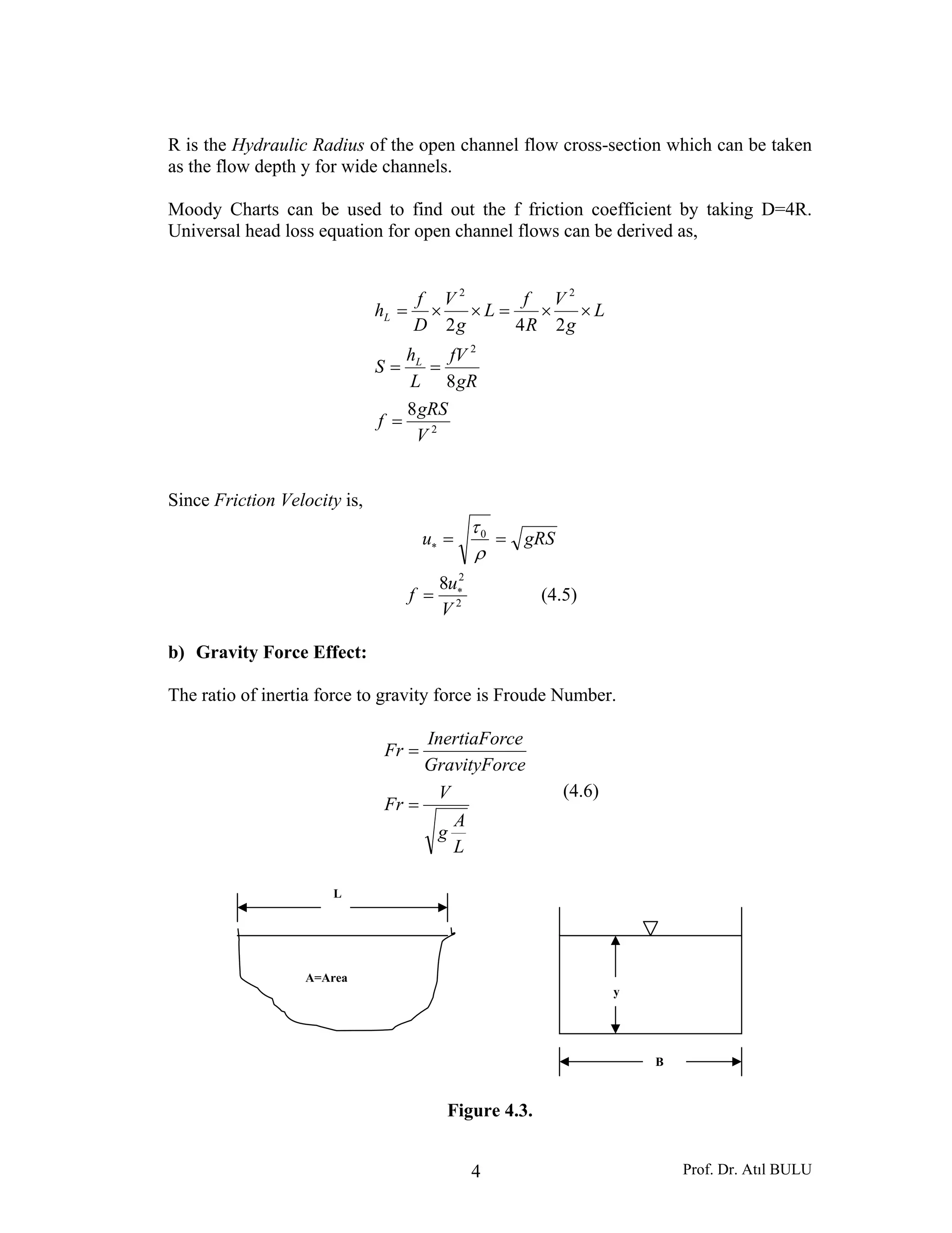
At the free surface [point 1 in Fig (4.5)] p1/ γ = 0 and z = z1, giving C = z1. At any point
A at a depth y below the free surface,
yp
yzz
p
A
A
A
γ
γ
=
=−= 1
(4.15)
This linear variation of pressure with depth with the constant of proportionality equal to
the specific weight of the liquid is known as hydrostatic pressure distribution.
4.5.2. Channels with Small Slope
Let us consider a channel with a very small value of the longitudinal slope θ. Let θ ≈ sinθ
≈1/1000. For such channels the vertical section is practically the same as the normal
section. If a flow takes place in this channel with the water surface parallel to the bed, the
streamlines will be straight lines and as such in a vertical direction [section 0 – 1 in Fig.
(4.6)] the normal acceleration an = 0. The pressure distribution at the section 0 – 1 will be
hydrostatic. At any point A at a depth y below the water surface,
y
p
=
γ
and 1zz
p
=+
γ
= Elevation of water surface
Figure 4. 6. Pressure distribution in a channel with small slope
Thus the piezometric head at any point in the channel will be equal to the water surface
elevation. The hydraulic grade line will therefore lie (coincide) on the water surface.
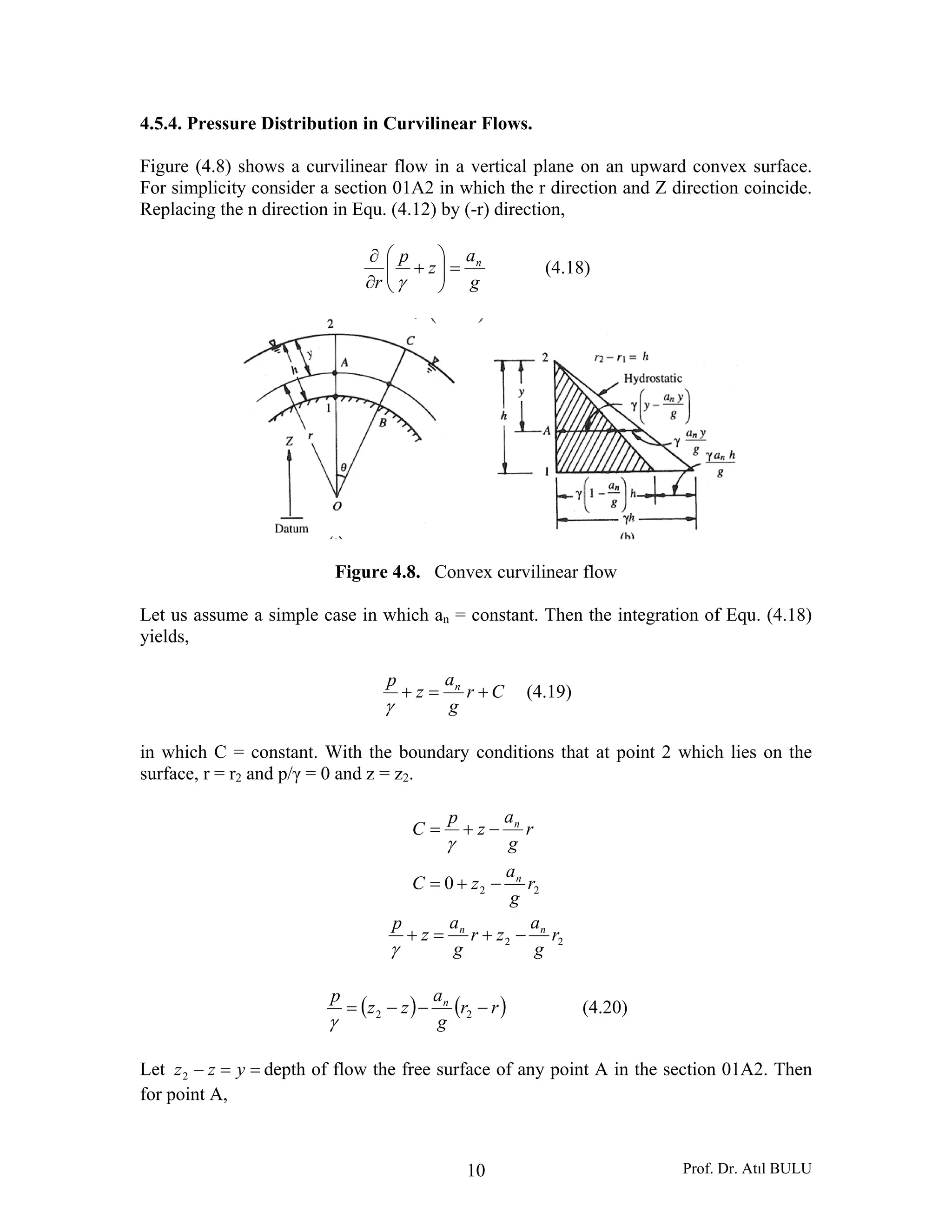
4.5.3. Channels with Large Slope
Fig. (4.7) shows a uniform free surface flow in a channel with a large value of inclination
θ. The flow is uniform, i.e. the water surface is parallel to the bed. An element of length
ΔL is considered at the cross-section 0 – 1.](https://image.slidesharecdn.com/lecturenotes04-160123205556/75/Open-Channel-Flows-Lecture-notes-04-8-2048.jpg)
![Prof. Dr. Atıl BULU11
( ) ( )zzyrr −==− 22
y
g
a
y
p n
−=
γ
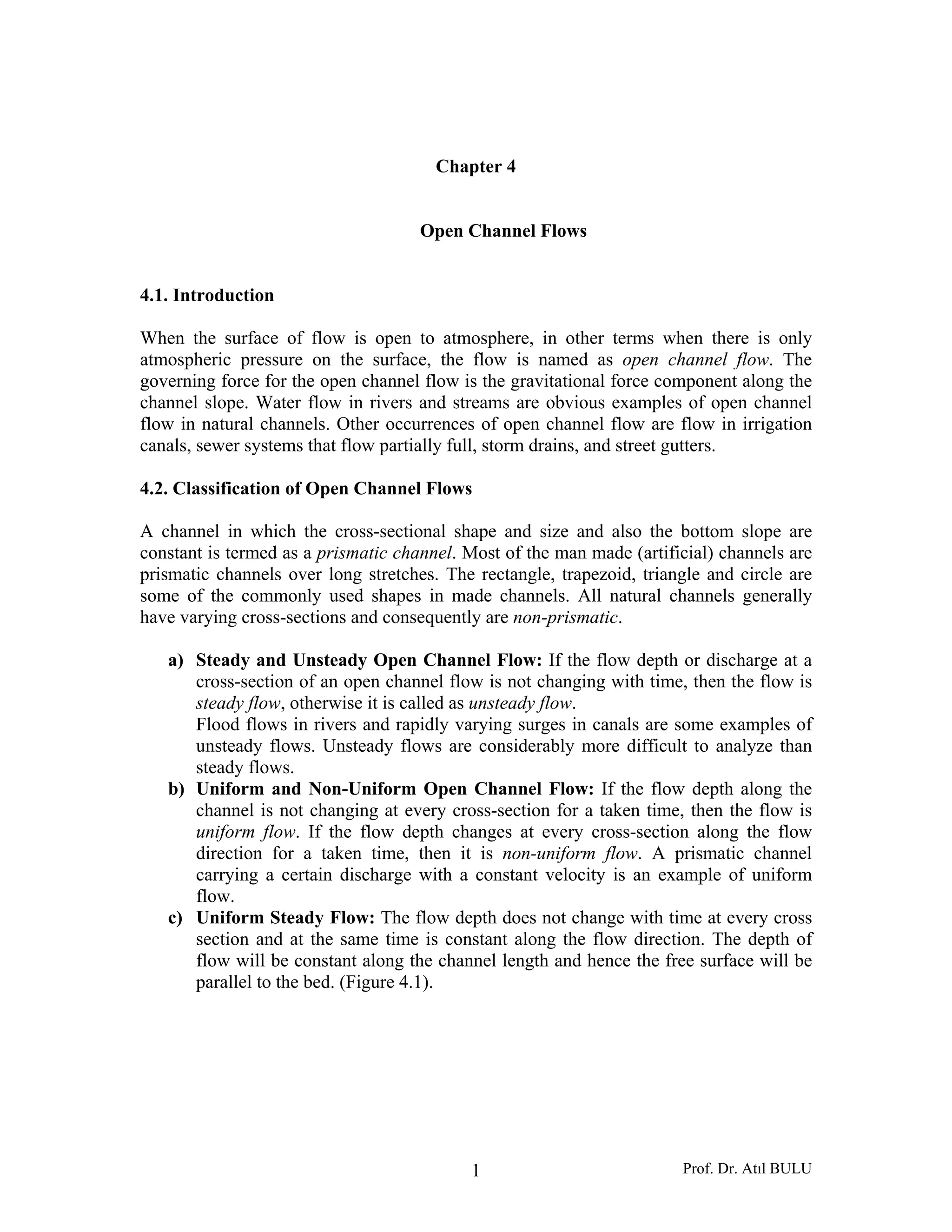
(4.21)
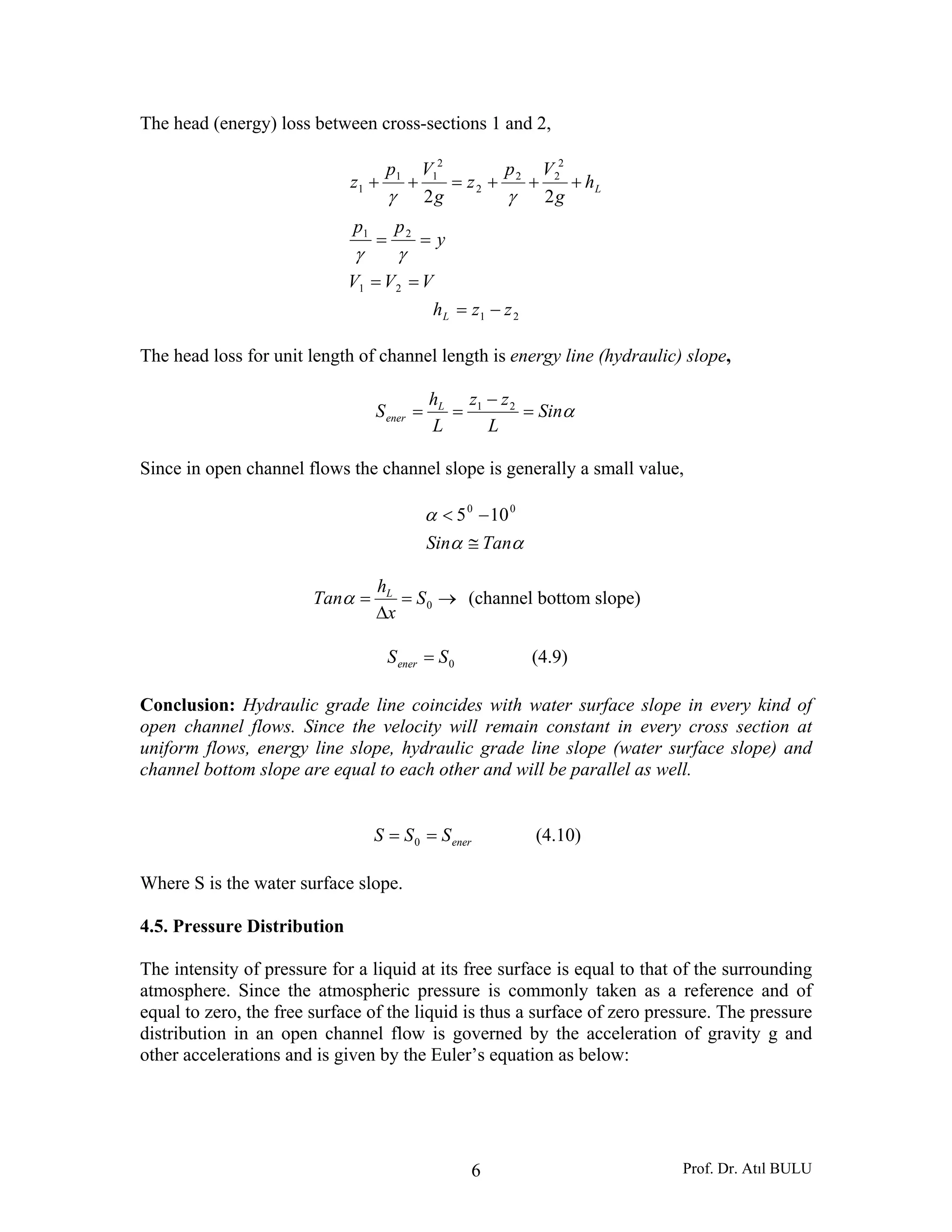
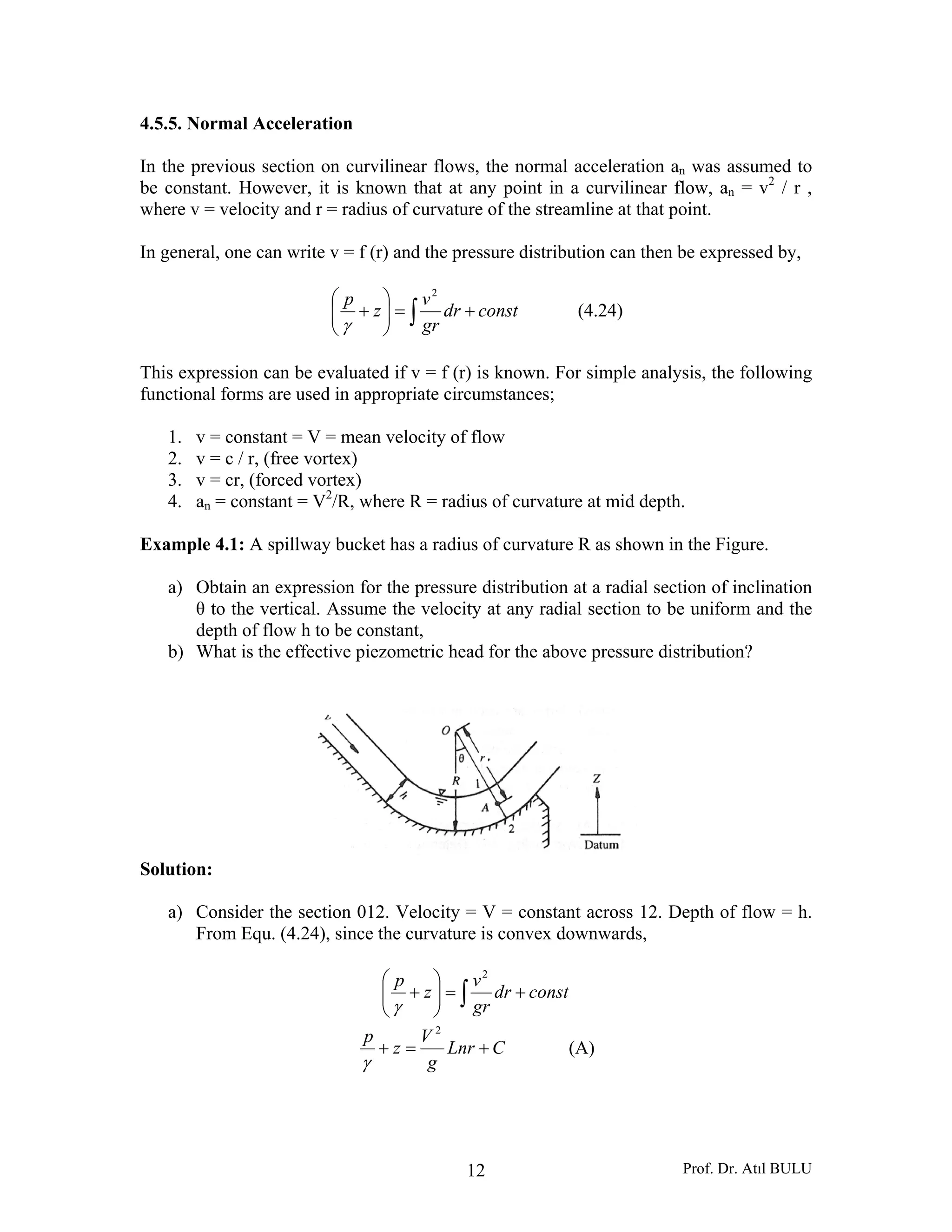
Equ. (4.21) shows that the pressure is less than the pressure obtained by the hydrostatic
distribution. Fig. (4.8).
For any normal direction OBC in Fig. (4.9), at point C, ( ) 0=Cp γ , 2rrC = , and for any
point at a radial distance r from the origin O,
( ) ( )
( ) θ
γ
cos2
2
rrzz
rr
g
a
zz
p
C
n
C
−=−
−−−=
( ) ( )rr
g
a
rr
p n
−−−= 22 cosθ
γ
(4.22)
If the curvature is convex downwards, (i.e. r direction is opposite to z direction)
following the argument above, for constant an the pressure at any point A at a depth y
below the free surface in a vertical section O1A2 [ Fig. (4.9)] can be shown to be,
y
g
a
y
p n
+=
γ
(4.23)
The pressure distribution in vertical section is as shown in Fig. (4.9)
Figure 4.8. Concave curvilinear flow
Thus it is seen that for a curvilinear flow in a vertical plane, an additional pressure will be
imposed on the hydrostatic pressure distribution. The extra pressure will be additive if the
curvature is convex downwards and subtractive if it is convex upwards.](https://image.slidesharecdn.com/lecturenotes04-160123205556/75/Open-Channel-Flows-Lecture-notes-04-11-2048.jpg)
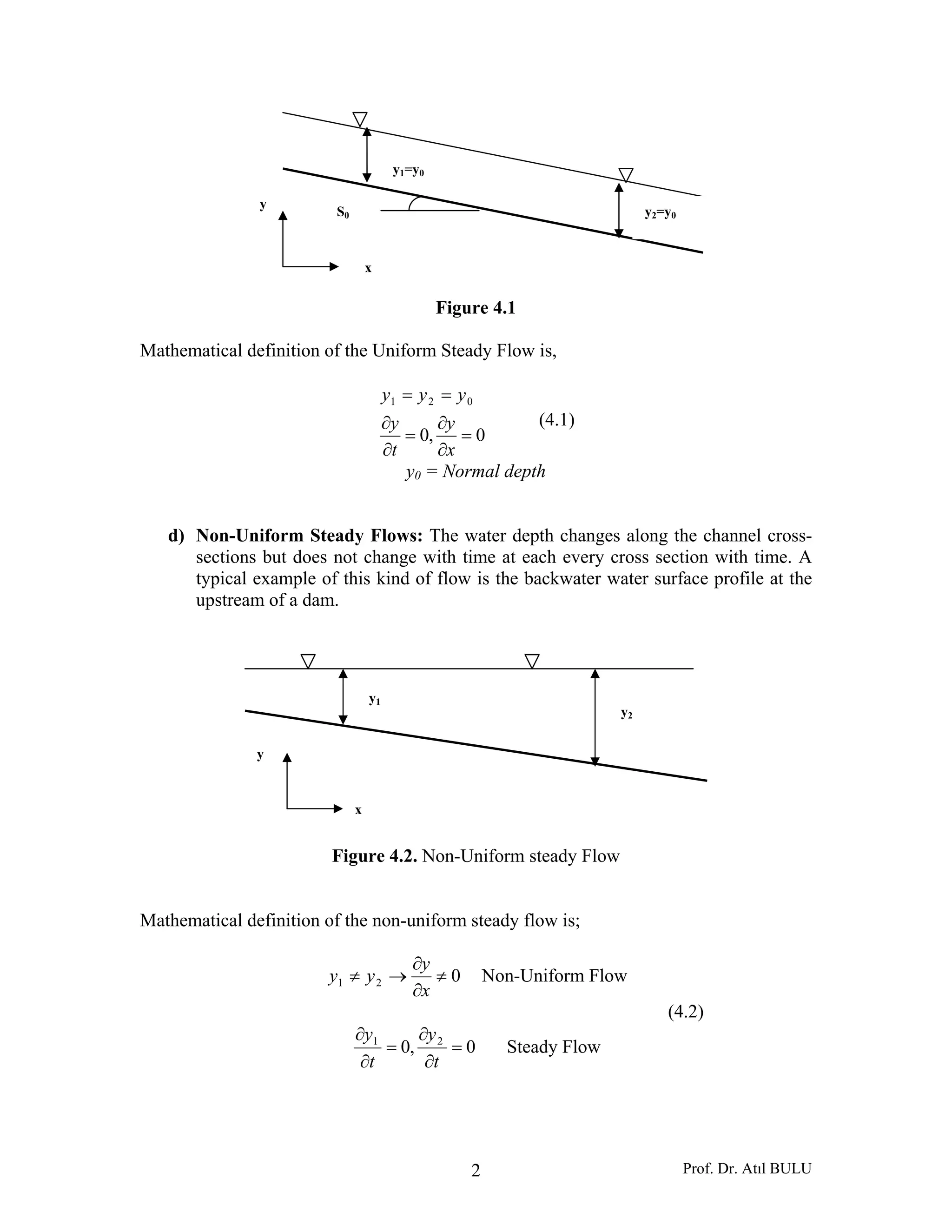
![Prof. Dr. Atıl BULU15
4) The force of resistance exerted by the bottom and sides of the channel cross-
section,
PLT 0τ=
w
Where P is wetted perimeter of the cross-section.
PLALSin
TFMWFM x
0
2211 0
τθγ =
=−−−++
wwwvvr
0
0
, SSinR
P
A
Sin
P
A
==
=
θ
θγτ
00 RSγτ = (4.25)
Using Equ. (4.5) and friction velocity equation,
0
2
0
2
2
2
2
0
8
8
8
RS
f
g
V
RS
fV
fV
U
U
×=
=
=
=
∗
∗
γρ
ρτ
0
8
RS
f
g
V ×= (4.26)
If we define,
0
8
RSCV
f
g
C
=
=
(4.27)
This cross-sectional mean velocity equation for open channel flows is known as Chezy
equation. The dimension of Chezy coefficient C,
[ ] [ ][ ] [ ]
[ ] [ ][ ][ ]
[ ] [ ]121
000211
21
0
21
−
−
=
=
=
TLC
TLFLCLT
SRCV](https://image.slidesharecdn.com/lecturenotes04-160123205556/75/Open-Channel-Flows-Lecture-notes-04-15-2048.jpg)
![Prof. Dr. Atıl BULU21
( )
∑
∑==
Pn
Pn
AAA
ii
i 23
23
( )
32
3223
P
Pn
n
ii∑= (4.35)
This equation gives a means of estimating the equivalent roughness of a channel having
multiple roughness types in its perimeters.
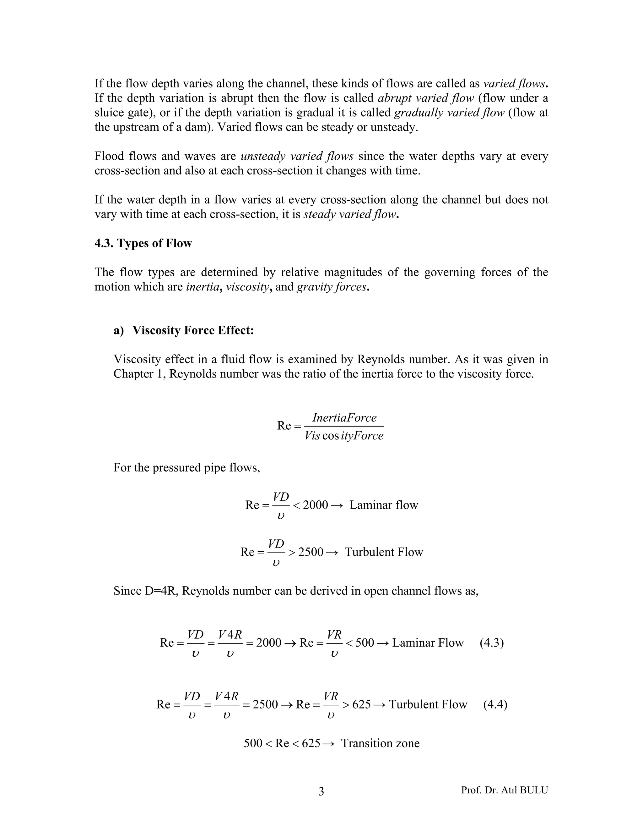
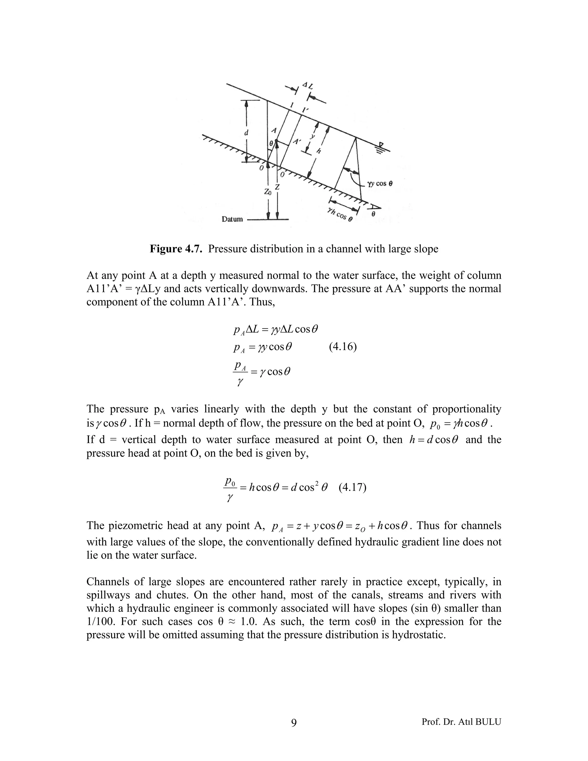
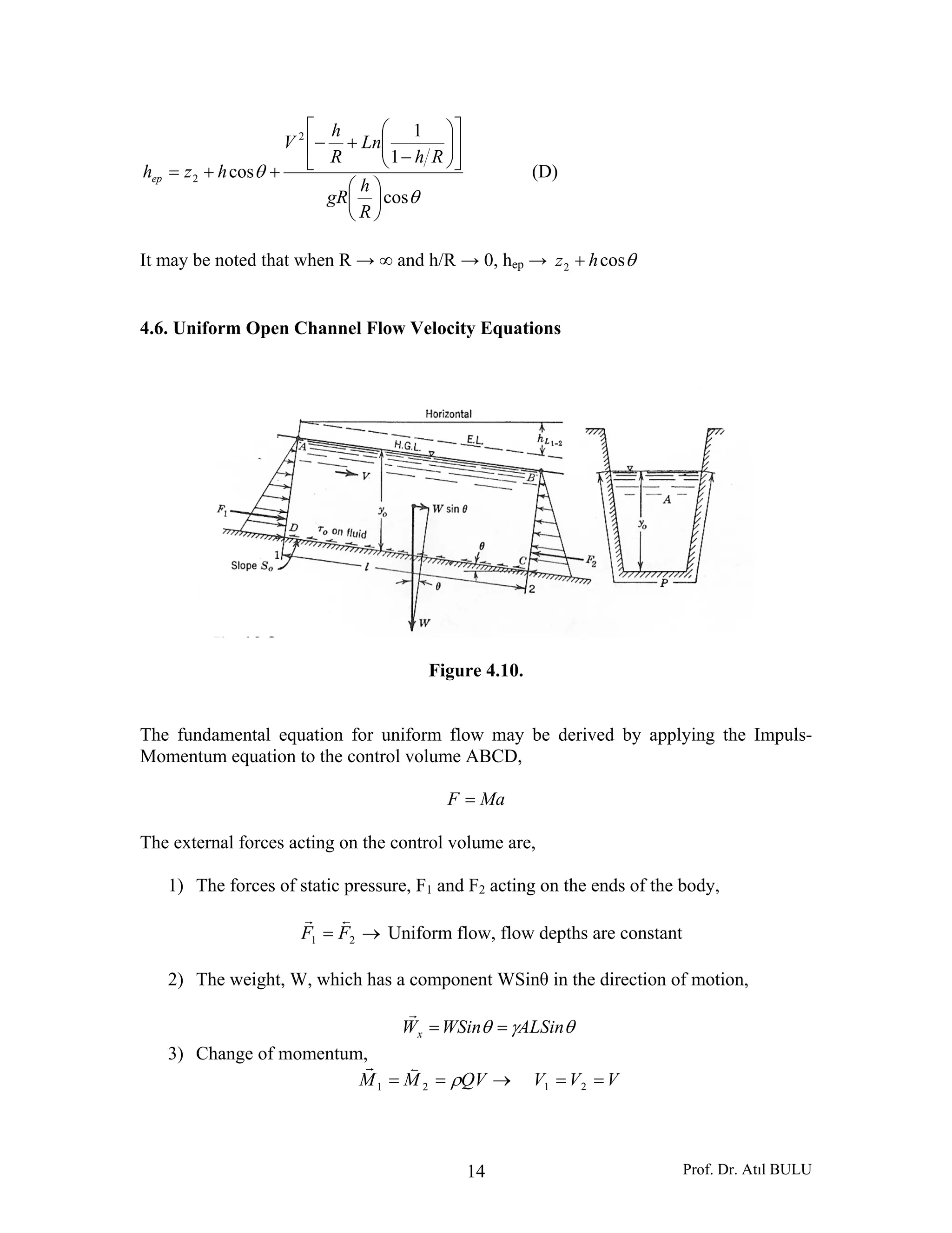
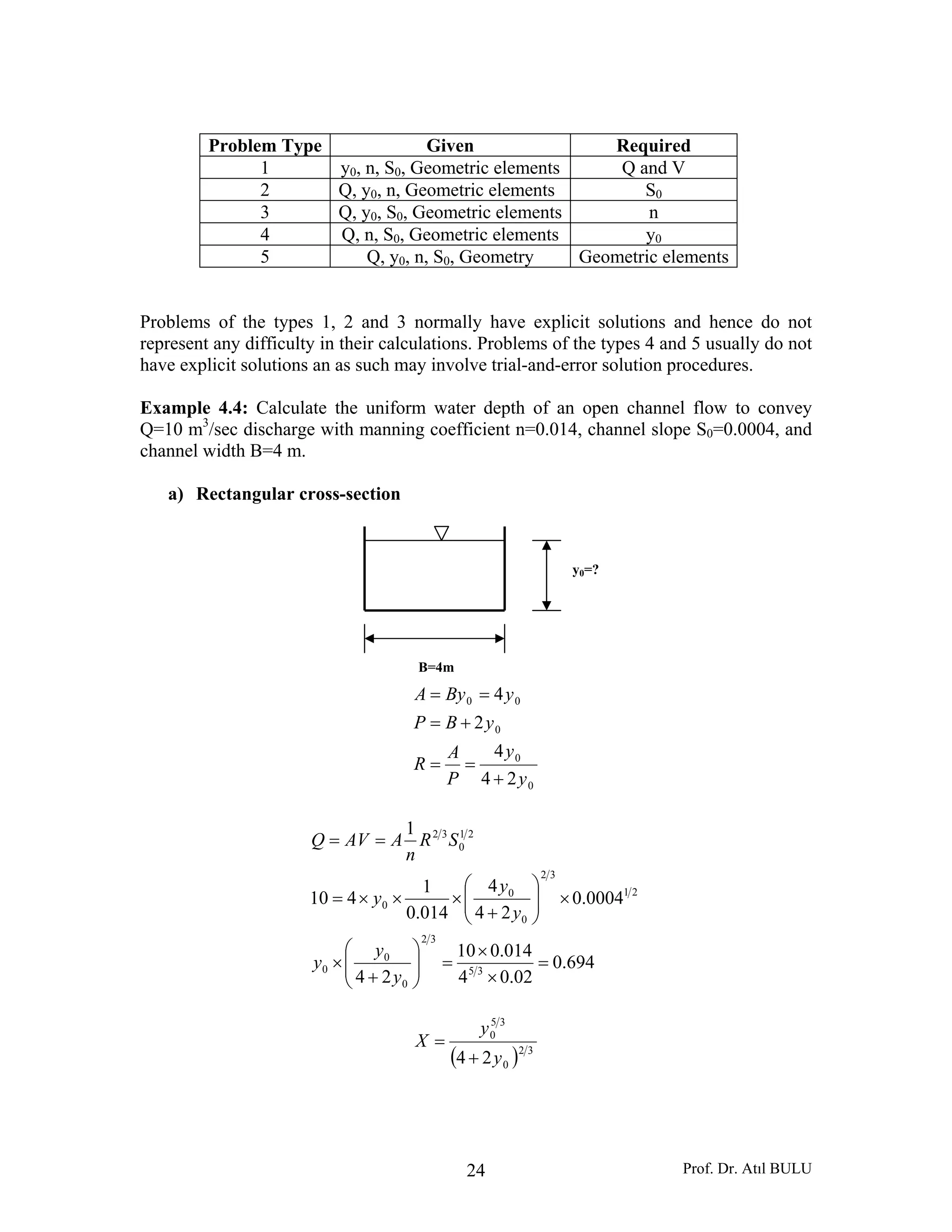
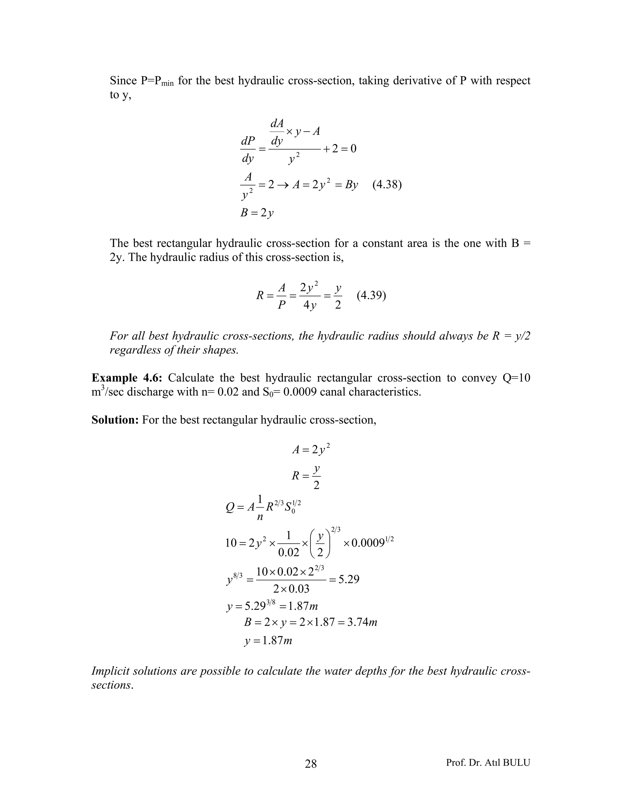
Example 4.3: An earthen trapezoidal channel (n = 0.025) has a bottom width of 5.0 m,
side slopes of 1.5 horizontal: 1 vertical and a uniform flow depth of 1.10 m. In an
economic study to remedy excessive seepage from the canal two proposals, a) to line the
sides only and, b) to line the bed only are considered. If the lining is of smooth concrete
(n = 0.012), calculate the equivalent roughness in the above two cases.
Solution:
Case a): Lining on the sides only,
For the bed → n1 = 0.025 and P1 = 5.0 m.
For the sides → n2 = 0.012 and mP 97.35.1110.12 2
2 =+××=
mPPP 97.897.30.521 =+=+=
Equivalent roughness, by Equ. (4.36),
[ ] 020.0
97.8
012.097.3025.00.5
32
325.15.1
=
×+×
=n
Case b): Lining on the bottom only,
P1 = 5.0 m → n1 = 0.012
P2 = 3.97 m → n2 = 0.025 →P = 8.97 m
( ) 018.0
97.8
025.097.3012.00.5
32
325.15.1
=
×+×
=n
1.5
1
1.1m
5m](https://image.slidesharecdn.com/lecturenotes04-160123205556/75/Open-Channel-Flows-Lecture-notes-04-21-2048.jpg)
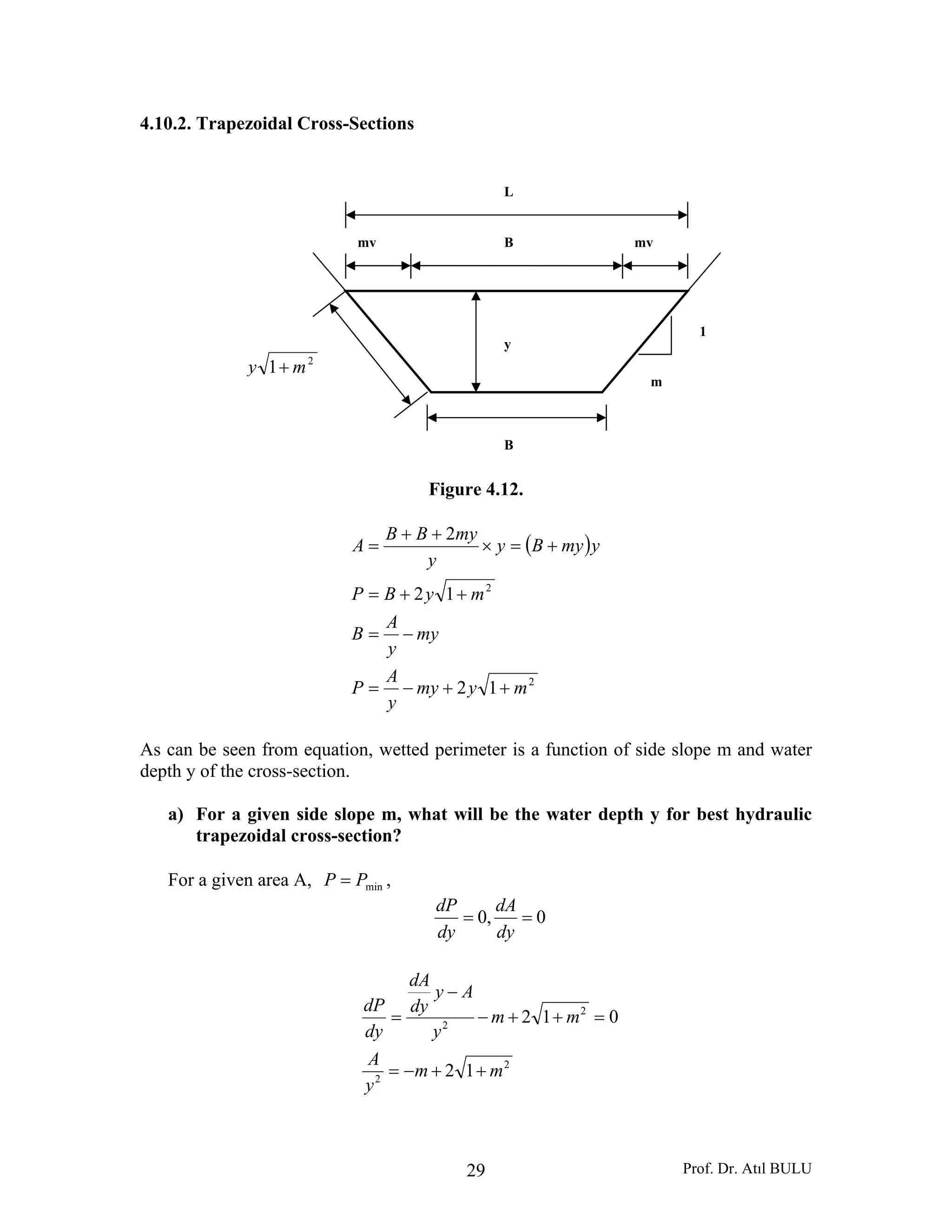

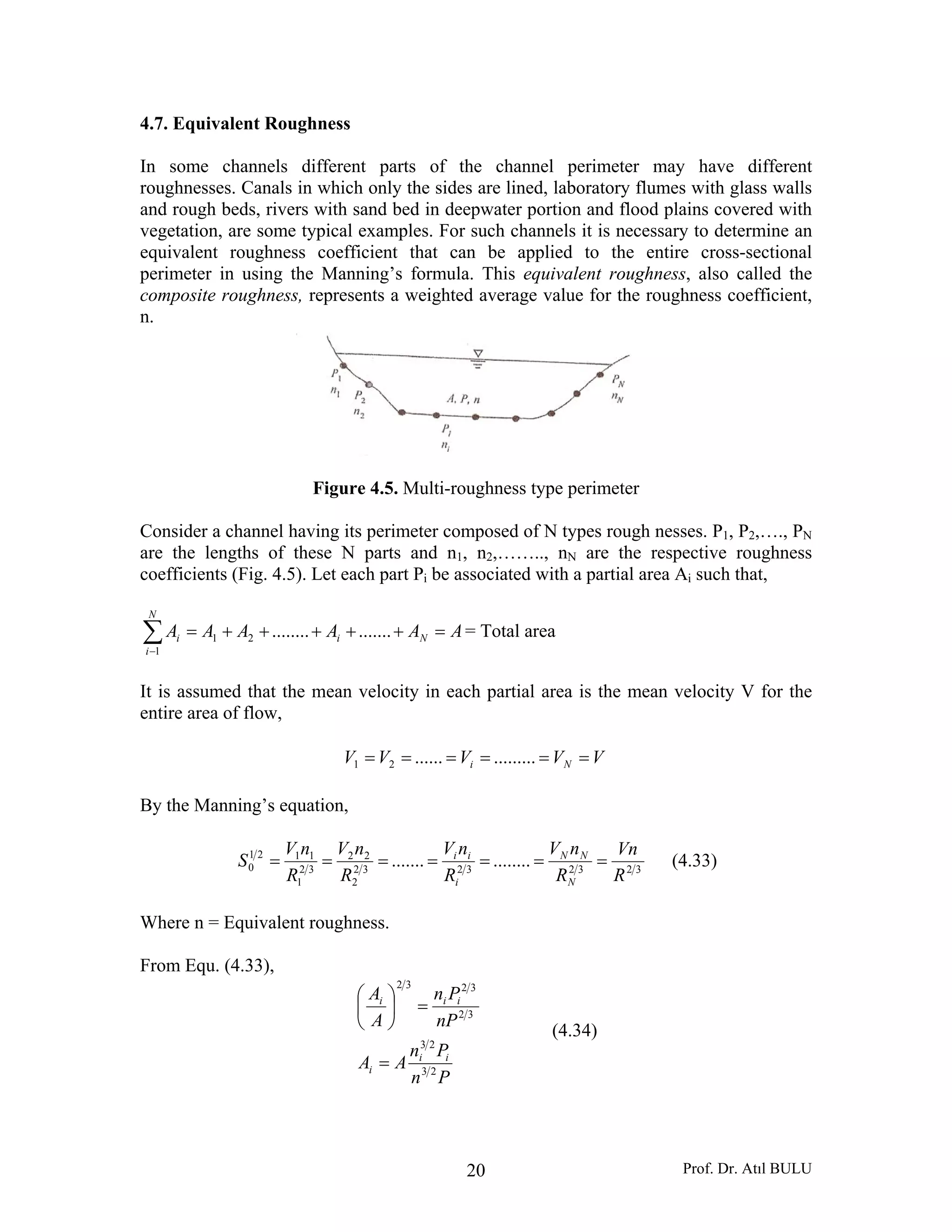
1) Open channel flow occurs when a surface of flow is open to the atmosphere, with only atmospheric pressure acting on the surface. Examples include rivers, streams, irrigation canals, and storm drains. 2) Open channel flows are classified based on whether the flow properties change over time (steady vs unsteady) or location (uniform vs non-uniform). Uniform steady flow has a constant depth at all locations and times. 3) The governing forces in open channel flows are inertia, viscosity, and gravity. Flow type is determined by the relative magnitudes of these forces, which can be laminar or turbulent depending on the Reynolds number, or subcritical or supercritical depending on the Froude number.


![Geotechnical Engineering-II [Lec #23: Rankine Earth Pressure Theory]](https://cdn.slidesharecdn.com/ss_thumbnails/23-181123050516-thumbnail.jpg?width=640&height=640&fit=bounds)