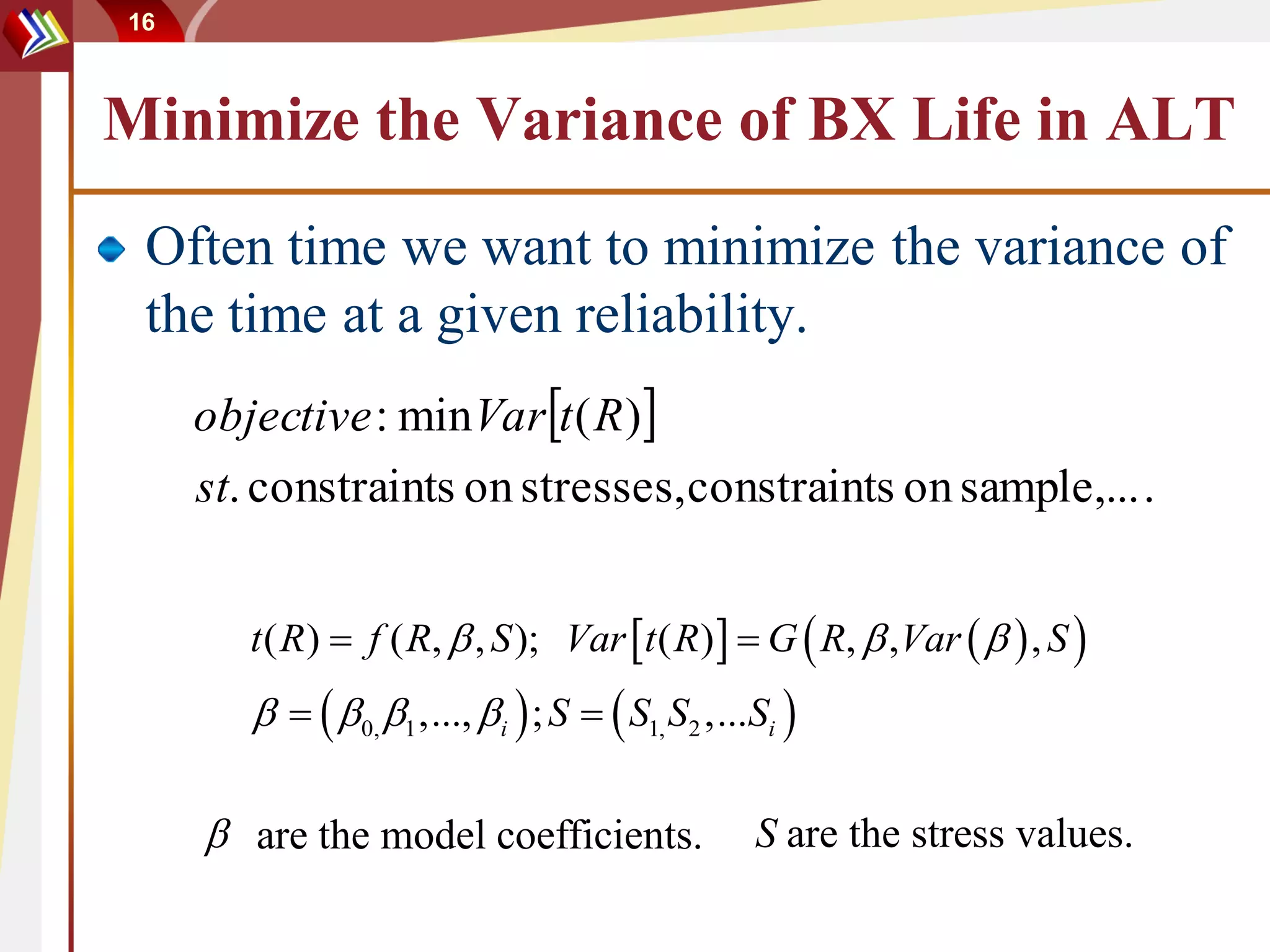
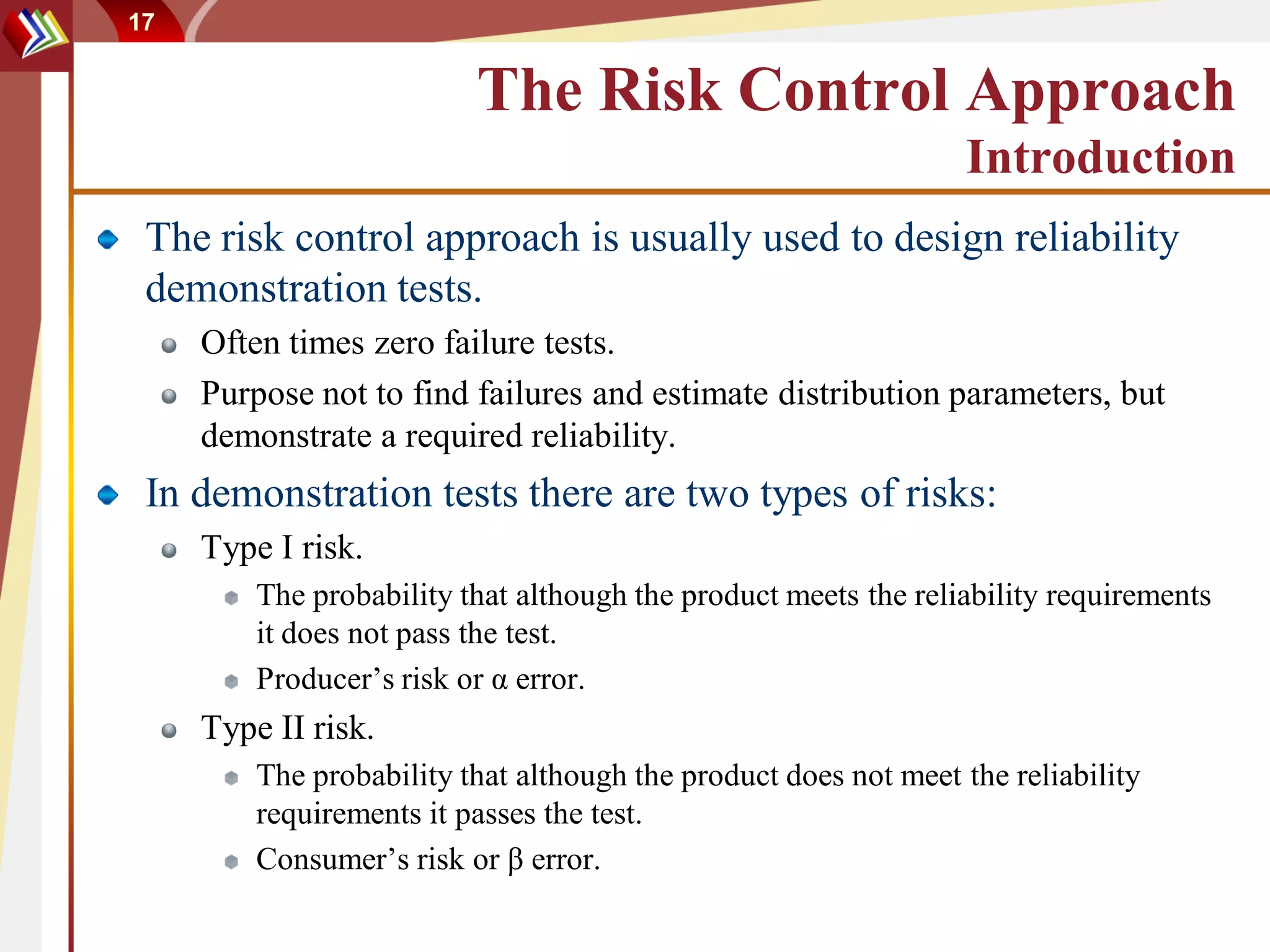
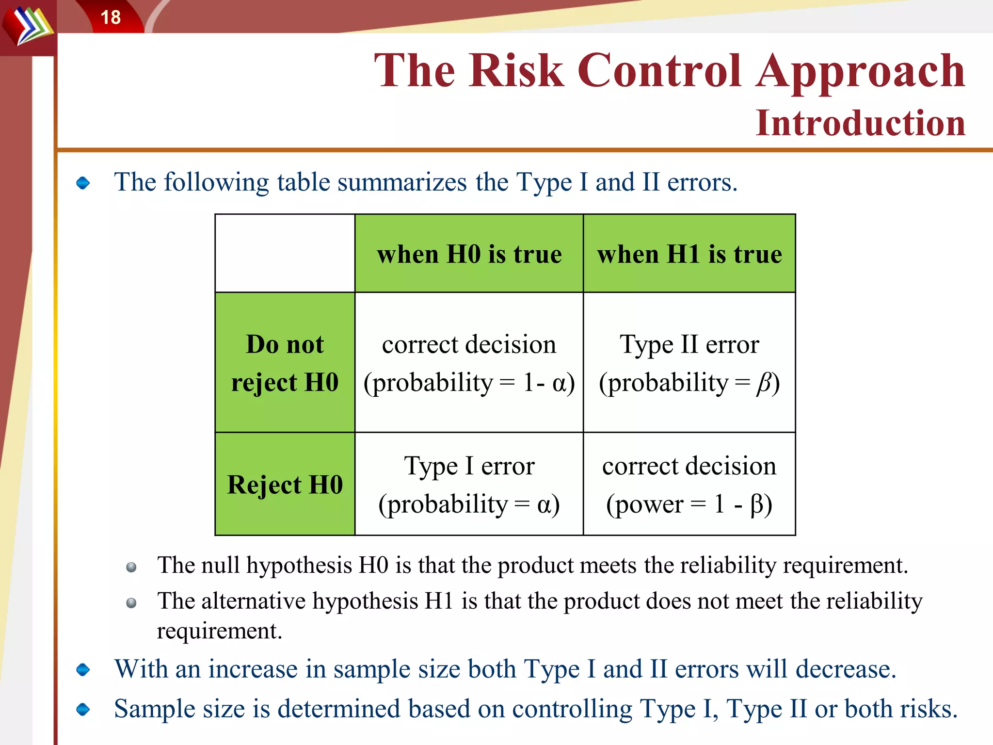
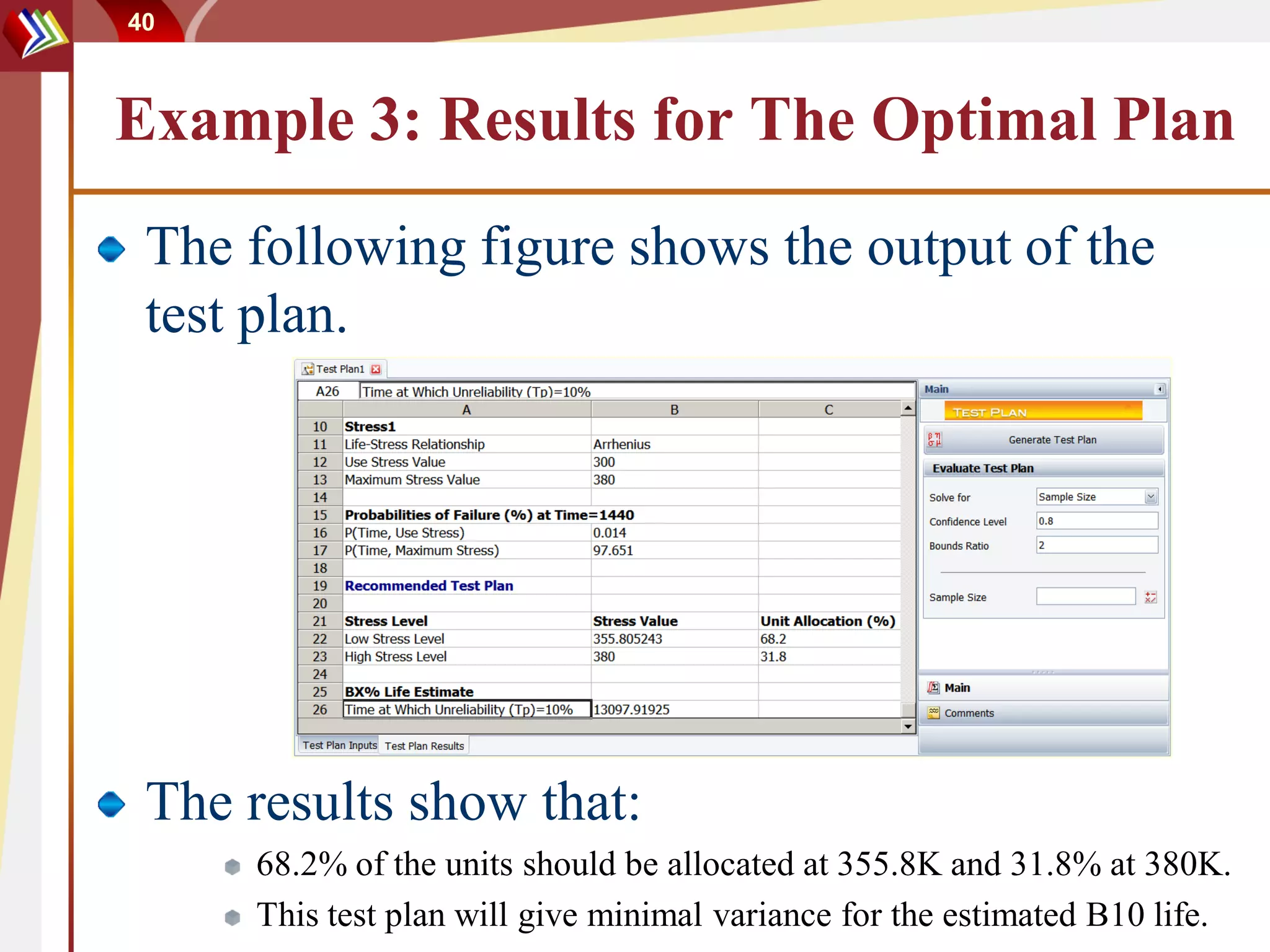
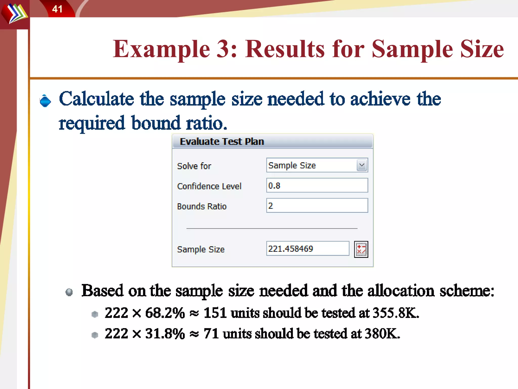
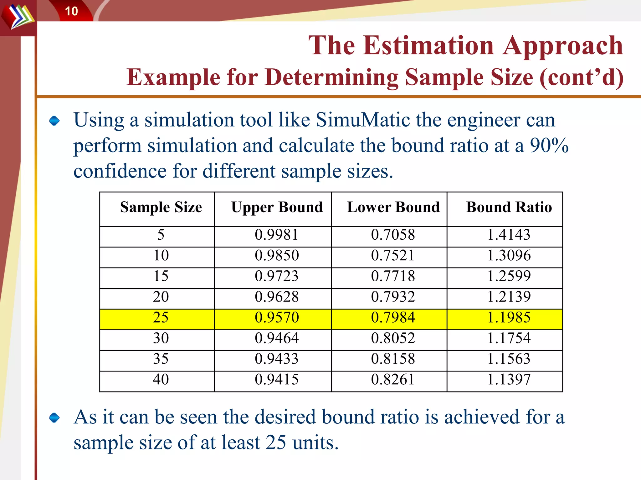
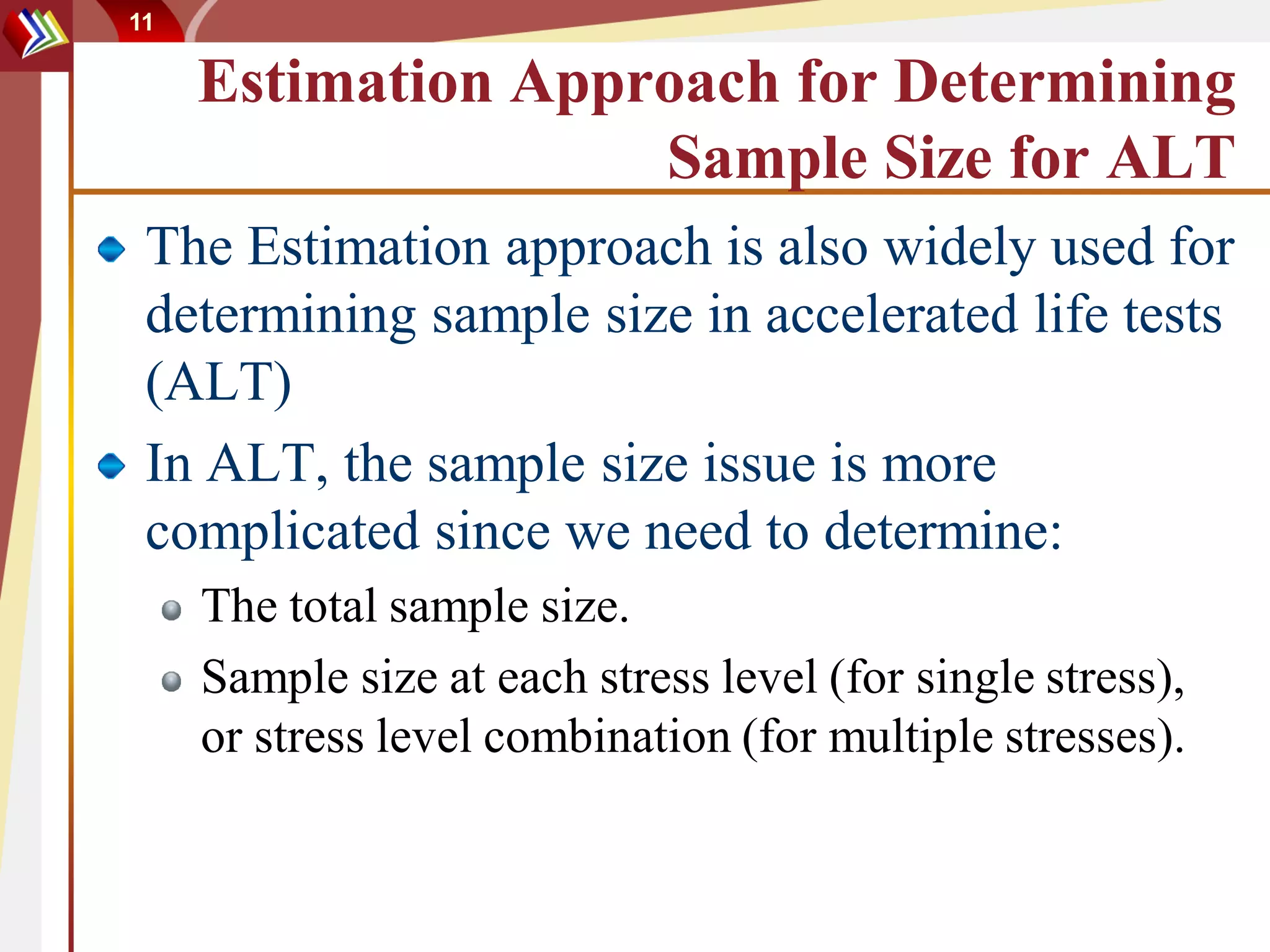
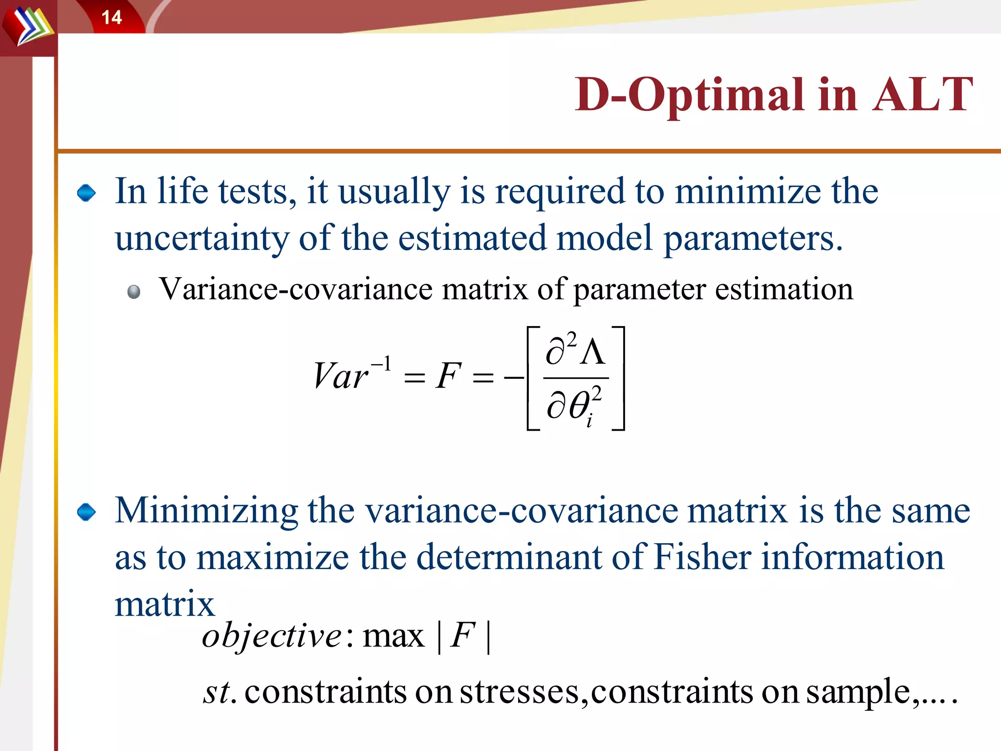
The document discusses methods for determining sample sizes in reliability testing. It covers two main approaches: the estimation approach which aims to control the confidence interval width, and the risk control approach which aims to control type I and type II errors. Examples are provided to demonstrate how to use each approach to determine the needed sample size given parameters like required reliability, confidence level, allowable failures. Both parametric and non-parametric methods are introduced for different test scenarios. Software tools can help calculate the sample sizes required to meet the test objectives.

1. Sample Size Issues on
Reliability Test Design
R li bilit T t D i
(可靠性试验设计中的样本量问
题)
Dr. Huairui Guo (郭怀瑞博士)
©2012 ASQ & Presentation Guo
Presented live on Sep 15th, 2012
http://reliabilitycalendar.org/The_Re
liability_Calendar/Webinars_
liability Calendar/Webinars ‐
_Chinese/Webinars_‐_Chinese.html

2. ASQ Reliability Division
ASQ Reliability Division
Chinese Webinar Series
Chinese Webinar Series
One of the monthly webinars
One of the monthly webinars
on topics of interest to
reliability engineers.
To view recorded webinar (available to ASQ Reliability
Division members only) visit asq.org/reliability
) /
To sign up for the free and available to anyone live
webinars visit reliabilitycalendar.org and select English
Webinars to find links to register for upcoming events
http://reliabilitycalendar.org/The_Re
liability_Calendar/Webinars_
liability Calendar/Webinars ‐
_Chinese/Webinars_‐_Chinese.html

3. 可靠性试验设计中的样本量
问题 (Sample Size Issues on
Reliability Test Design)
郭怀瑞, Ph.D., CRE, CQE, CRP
©1992-2012 ReliaSoft Corporation - ALL RIGHTS RESERVED

4. 2
Outlines
Part 1: Methods for determining sample size
Parameter estimation based approaches
Risk control based approaches
Part 2: Examples using software tools from
ReliaSoft

5. 3
EDUCATION
Part I: Methods for Determining Sample
Sizes in Reliability Tests

6. 4
Sample Size Issues on Reliability Test Design
Introduction
One of the most critical questions when
designing a reliability test is determining the
appropriate sample size.
If sample size is too large, unnecessary costs
may be incurred.
If sample size too small, the uncertainty of the
reliability estimates will be unacceptably high.

7. 5
Sample Size Issues on Reliability Test Design
Introduction (cont’d)
Two methods in determining the required sample size:
The Estimation Approach (similar to the alphabetic optimal
criteria)
The goal is to determine the effect of sample size on confidence
intervals (variance).
Sample size is determined based on the desired confidence interval
width.
The Risk Control Approach
The goal is to control the Type I and Type II errors.
This is also referred to as power and sample size in design of
experiments (DOE).

8. 6
The Estimation Approach
Effect of Sample Size on Confidence Interval
From historical information an engineer knows that
component’s life follows a Weibull distribution with:
beta=2.3
eta=1,000 hours.
The engineer first wants to see how the sample
size affecting the confidence bounds of the
estimated reliabilities.

9. 7
The Estimation Approach
Effect of Sample Size on Interval Width
The following plot shows the simulation bounds for a sample size of 5 units.
ReliaSof t W eibull+ + 7 - www. ReliaSoft. com
Probability - Weibull
99. 000
Weibull-2P
MLE SRM MED FM
F=0/ S=0
90. 000 True Parameter Line
Top CB-R
Bottom CB-R
50. 000
U n r e lia b ilit y , F ( t )
10. 000
5. 000
Harry Guo
Reliasoft
6/ 7/ 2012
2:31:21 PM
1. 000
100. 000 1000. 000 10000. 000
Time, (t)
            

10. 8
The Effect of Sample Size on Interval Width
(cont’d)
The following plot shows the simulation bounds for a sample size of 40 units.
ReliaSof t W eibull+ + 7 - www. ReliaSoft. com
Probability - Weibull
99. 000
Weibull-2P
MLE SRM MED FM
F=0/ S=0
90. 000 True Parameter Line
Top CB-R
Bottom CB-R
50. 000
U n r e lia b ilit y , F ( t )
10. 000
5. 000
Harry Guo
Reliasoft
6/ 7/ 2012
2:32:52 PM
1. 000
100. 000 1000. 000 10000. 000
Time, (t)
            

11. 9
The Estimation Approach
Example for Determining Sample Size
Therefore, sample size can be determined based
on the required of the width of the estimated
confidence bounds.
For the above example, determine the needed
sample size so that the ratio of the upper bound
to the lower bound of the estimated reliability at
400 hours is less than 1.2 at a confidence level
of 90%.

12. 10
The Estimation Approach
Example for Determining Sample Size (cont’d)
Using a simulation tool like SimuMatic the engineer can
perform simulation and calculate the bound ratio at a 90%
confidence for different sample sizes.
Sample Size Upper Bound Lower Bound Bound Ratio
5 0.9981 0.7058 1.4143
10 0.9850 0.7521 1.3096
15 0.9723 0.7718 1.2599
20 0.9628 0.7932 1.2139
25 0.9570 0.7984 1.1985
30 0.9464 0.8052 1.1754
35 0.9433 0.8158 1.1563
40 0.9415 0.8261 1.1397
As it can be seen the desired bound ratio is achieved for a
sample size of at least 25 units.

13. 11
Estimation Approach for Determining
Sample Size for ALT
The Estimation approach is also widely used for
determining sample size in accelerated life tests
(ALT)
In ALT, the sample size issue is more
complicated since we need to determine:
The total sample size.
Sample size at each stress level (for single stress),
or stress level combination (for multiple stresses).

14. 12
Optimal Design Criteria in Design of
Experiments (DOE)
x1 x2 x3
 1 1  1
X   1 1  1
 
 .. .. .. 
 

15. 13
Distributions and Models in ALT
Failure time distribution
Exponential
Weibull
Lognormal
Life-stress model
log(t )  0  1 x1  2 x2  ...  
Maximum likelihood estimation
 f (ti ) if the ith observation is an exact failure

li   F (ti ,U )  F (ti , L ) if the ith observation is an interval failure
 R( s ) if the ith observation is an suspension
 i
n
  ln( L )   li
i 1

16. 14
D-Optimal in ALT
In life tests, it usually is required to minimize the
uncertainty of the estimated model parameters.
Variance-covariance matrix of parameter estimation
  2 
Var 1  F    2 
 i 
Minimizing the variance-covariance matrix is the same
as to maximize the determinant of Fisher information
matrix
objective : max | F |
st. constraints on stresses, constraints on sample,... .

17. 15
Example: Time-Censored ALT with 2
Stresses
Log-likelihood function si 
  ( 0  1 X i ,1   2 X i , 2  12 X i ,1 X i , 2 )

 1 zi2, j  1 Yij  
li , j (  ,  )  I ij   ln   ln 2 

  (1  I ij ) ln(1   ( si )) if
 2 2  
I ij  
0 if Yij  
E[ I ij ]  ( si )
Fisher information matrix
n A n x A n x A n x x A
i i i i ,1 i i i ,2 i i i ,1 i ,2 i n A  si i i i
n A n x x A n x A
i i i i ,1 i ,2 i i i ,2 i n A  s x
i i i i i ,1
F
1 n A n x A i i i i ,1 i n A  s x
i i i i i ,2
  i 
2
n A i i n A  s x x
i i i i i ,1 i ,2
Ai   i  i  si  
 1  i 
   s 
 
 n 2
i

i  i si  si2  1  i i  
1  i 
i   
Find ni to maximize |F|. Planned distribution
parameter values are needed

18. 16
Minimize the Variance of BX Life in ALT
Often time we want to minimize the variance of
the time at a given reliability.
objective : min Vart ( R )
st. constraints on stresses, constraints on sample,... .
t ( R)  f ( R,  , S ); Var t ( R)   G  R,  ,Var    , S 
   0, 1 ,..., i  ; S   S1, S2 ,...Si 
 are the model coefficients. S are the stress values.

19. 17
The Risk Control Approach
Introduction
The risk control approach is usually used to design reliability
demonstration tests.
Often times zero failure tests.
Purpose not to find failures and estimate distribution parameters, but
demonstrate a required reliability.
In demonstration tests there are two types of risks:
Type I risk.
The probability that although the product meets the reliability requirements
it does not pass the test.
Producer’s risk or α error.
Type II risk.
The probability that although the product does not meet the reliability
requirements it passes the test.
Consumer’s risk or β error.

20. 18
The Risk Control Approach
Introduction
The following table summarizes the Type I and II errors.
when H0 is true when H1 is true
Do not correct decision Type II error
reject H0 (probability = 1- α) (probability = β)
Type I error correct decision
Reject H0
(probability = α) (power = 1 - β)
The null hypothesis H0 is that the product meets the reliability requirement.
The alternative hypothesis H1 is that the product does not meet the reliability
requirement.
With an increase in sample size both Type I and II errors will decrease.
Sample size is determined based on controlling Type I, Type II or both risks.

21. 19
The Risk Control Approach
Non-Parametric Binomial for Demonstration Tests

22. 20
The Risk Control Approach
Non-Parametric Binomial for Demonstration Tests
In the Non-Parametric Binomial equation time is not a
factor.
The Non-Parametric method is used:
For one-shot devices where time is not a factor.
For cases when the test time is the same as the time at which
we require the demonstrated reliability.
When time is a factor, the so called parametric
Binomial should be used, and a failure time
distribution is assumed.

23. 21
The Risk Control Approach
Example
A reliability engineer wants to design a zero
failure demonstration test.
The target reliability is 80% at 100 hours.
The required confidence level is 90% (the Type
II error is 10%).
The available test time is 100 hours.
What is the required sample size?

24. 22
The Risk Control Approach
Solution

25. 23
The Risk Control Approach
Example: Solution (cont’d)
If 1 out the 11 samples in the test fails, the
demonstrated reliability will be less than the
required.
In this case it will be:

26. 24
The Risk Control Approach
Exponential Chi-Squared Demonstration Test

27. 25
The Risk Control Approach
Example
We want to design a test in order to
demonstrate:
An 85% reliability at 500 hours.
With a 90% confidence.
Only up to two failures are allowed in the test.
The assumed distribution is exponential.
The available test duration is 300 hours.
Determine the sample size needed.

28. 26
The Risk Control Approach
Example: Solution

29. 27
The Risk Control Approach
Example: Solution (cont’d)
Using Weibull++, the total accumulated test time based on the
available test time and required sample size is:

30. 28
The Risk Control Approach
Non-Parametric Bayesian Test
Bayesian methodology utilizes historical
information to improve “accuracy”.
In reliability testing, Bayesian methods can be
beneficial when:
Available sample size is small.
Prior information on the product’s reliability is
available.

31. 29
The Risk Control Approach
Non-Parametric Bayesian Test (cont’d)

32. 30
The Risk Control Approach
Non-Parametric Bayesian Test (cont’d)

33. 31
The Risk Control Approach
Bayesian Test With Subsystem Information

34. 32
The Risk Control Approach
Bayesian Test With Subsystem Information (cont’d)

35. 33
The Risk Control Approach
Example
Assume a system of interest is composed of three subsystems
A, B and C.
The following table shows prior subsystem test results.
What is the required sample size in order to demonstrate:
A system reliability of 90% at an 80% confidence level.
With 1 allowed failure in the test.

36. 34
The Risk Control Approach
Example: Solution
The following figure shows the results of the
Bayesian test design.

37. 35
EDUCATION
Part II: Examples of Using
Software Tools

38. 36
Example 1: Non-Parametric Binomial
A reliability engineer had the following informaiton from a
reliability demonstration test.
50 Samples are tested for 100 hours and 1 failure was observed.
What is the demonstrated reliability at a confidence level of 80%?

39. 37
Example 2: Parametric Binomial
Design a test to demonstrate the reliability of 80% at 2,000 hours with a 90%
confidence.
The available test time is 1,500 hours.
The maximum allowed failures in the test are 1.
It is assumed that the component follows a Weibull distribution with beta of 2.
What is the required sample size?

40. 38
Example 3: One Stress ALT
A reliability engineer wants to design an ALT for an
electronic component.
Use temperature is 300K while design limit is 380K.
The engineer has:
2 months or 1,440 hours available for testing and 2 available chambers.
From historical data:
The beta parameter of the Weibull distribution is 3.
The probability of failure at use temperature at time 1,440 is 0.00014, at
the design limit is 0.97651.
The engineer wants to determine:
The appropriate temperature that should be set at each chamber.
The number of units that should be allocated at each chamber.

41. 39
Example 3: One Stress ALT
The sample size should be such that the bound ratio for the
estimated B10 life is 2 at the 80% confidence level.
The inputs for a 2 Level Statistically Optimum Test Plan is

42. 40
Example 3: Results for The Optimal Plan
The following figure shows the output of the
test plan.
The results show that:
68.2% of the units should be allocated at 355.8K and 31.8% at 380K.
This test plan will give minimal variance for the estimated B10 life.

43. 41
Example 3: Results for Sample Size

44. 42
Where to Get More Information
1. http://www.itl.nist.gov/div898/handbook/
2. www.Weibull.com
3. http://www.reliawiki.org/index.php/ReliaSoft_Books