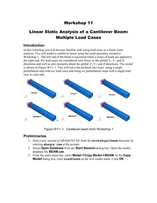
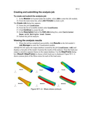
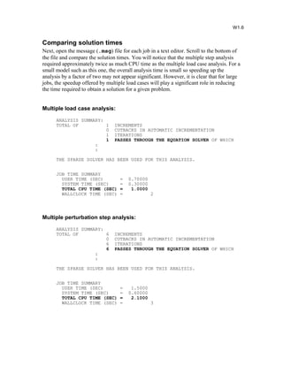
Workshop 11
Linear Static Analysis of a Cantilever Beam:
Multiple Load Cases
Introduction
In this workshop you will become familiar with using load cases in a linear static
analysis. You will model a cantilever beam using the same geometry created in
Workshop 1. The left end of the beam is encastred while a series of loads are applied to
the right end. Six load cases are considered: unit forces in the global X-, Y-, and Z-
directions and well as unit moments about the global X-, Y-, and Z-directions. The model
is shown in Figure W11–1. You will solve the problem two ways: using a single
perturbation step with six load cases and using six perturbation steps with a single load
case in each step.
Figure W11–1. Cantilever beam from Workshop 1
Preliminaries
1. Start a new session of ABAQUS/CAE from the workshops/beam directory by
entering abaqus cae at the prompt.
2. Select Open Database from the Start Session dialog box. Open the model
database file BEAM.cae.
3. From the main menu bar, select ModelCopy ModelBEAM. In the Copy
Model dialog box, enter LoadCases as the new model name. Click OK.
Defining a linear perturbation static step
1. Switch to the Step module.
2. From the main menu bar, select StepDeleteBeamLoad to delete
the general static step created in Workshop 1. ABAQUS warns you that
deleting a step also deletes other model attributes such as output requests
and loads that are defined in the step. Click Yes to accept this.
The general static step will now be replaced by a linear perturbation static step.
3. From the main menu bar, select StepCreate to create a step.
4. Name the step LoadCases.
5. From the list of available Linear perturbation procedures in the
Create Step dialog box, select Static, Linear Perturbation and click
Continue.
6. In the Description field of the Basic tabbed page, type Six load
cases applied to right end of beam.
7. Click OK to create the step and to exit the step editor.
Defining a rigid body constraint to transmit the load
As indicated in Figure W11–1, we wish to apply forces and moments to the right end of
the beam. However, the beam is modeled with solid C3D8I elements, which possess only
displacement degrees of freedom. Thus, only forces may be directly applied to the model.
Rather than applying force couples to the model, we will apply concentrated moments to
the end of the beam. To this end, all loads will be transmitted to the beam through a rigid
body constraint. This approach is adopted to take advantage of the fact that the rigid body
reference point possesses six degrees of freedom in three-dimensions: 3 translations and
3 rotations and thus allows direct application of concentrated moments. Rigid bodies and
constraints will be discussed further in Lecture 12.
To create a rigid body constraint:
1. In the Module list located under the toolbar, select Interaction to enter the
Interaction module.
4. From the main menu bar, select ToolsReference Point to create a reference
point for the rigid body constraint. The reference point should be placed at the
center of the right end of the beam. The coordinates are 100.0, 0.0, 12.5.
5. From the main menu bar, select ConstraintCreate to create a rigid body
constraint. In the Create Constraint dialog box, select Rigid body as the
constraint type and click Continue.
6. In the Edit Constraint dialog box, select Pin (nodes) as the Region type
and click Edit on the right side of the editor. In the viewport, select the face at the
right end of the beam as the pin region for the rigid body. When you have selected
this face, click Done in the prompt area.
7. In the bottom half of the editor, click Edit to edit the Reference Point and
select the reference point created earlier as the rigid body reference point.
8. Click OK to close the Edit Constraint dialog box.
W1.2
Defining loads and load cases
To define loads:
1. In the Module list located under the toolbar, select Load to enter the
Load module.
9. From the main menu bar, select LoadCreate.
10. In the Create Load dialog box:
A. Name the load Force-X.
A. Select LoadCases as the step in which the load will be activated.
B. In the Category list, accept Mechanical as the default category selection.
C. In the Types for Selected Step list, select Concentrated force as the
type and click Continue.
D. Select the reference point as the point to which the load will be applied.
E. In the Edit Load dialog box, enter a value of 1.0 for CF1.
F. Click OK to close the dialog box.
11. Similarly, create two additional Concentrated force loads named Force-Y
and Force-Z and three Moment loads named Moment-X, Moment-Y, and
Moment-Z.
A. For loads Force-Y and Force-Z, set CF2=1.0 and CF3=1.0, respectively.
B. For loads Moment-X, Moment-Y, and Moment-Z, set CM1=1.0,
CM2=1.0, and CM3=1.0, respectively.
ABAQUS/CAE displays arrows at the reference point indicating the loads applied to the
model.
To define load cases:
1. From the main menu bar, select Load CaseCreate.
The Create Load Case dialog box appears.
12. In the Create Load Case dialog box:
A. Name the load case LC-Force-X, select LoadCases as the step, and click
Continue.
G. In the Edit Load Case dialog box, select the Loads tabbed page and click
Add.
H. In the Load Selection dialog box, select Force-X and click OK.
I. Click OK to close the Edit Load Case dialog box.
13. Repeat this procedure to create five additional load cases: one for each of the
remaining loads. Name the load cases LC-Force-Y, LC-Force-Z, LC-
Moment-X, LC-Moment-Y, and LC-Moment-Z and add the corresponding
load to each.
Note that the fixed-end boundary conditions were defined in the initial step, and as such,
are active in each load case of the analysis step.
W1.3
Creating and submitting the analysis job
To create and submit the analysis job:
1. In the Module list located under the toolbar, select Job to enter the Job module.
14. From the main menu bar, select JobCreate to create a job.
The Create Job dialog box appears.
15. Name the job loadCases.
16. From the list of available models select LoadCases.
17. Click Continue to create the job.
18. In the Description field of the Edit Job dialog box, enter Cantilever
Beam with Multiple Load Cases.
19. Submit the job for analysis.
Viewing the analysis results
1. When the job has completed successfully, click Results in the Job module’s
Job Manager to enter the Visualization module.
ABAQUS/CAE opens the output database created by the job (loadCases.odb) and
displays a fast plot of the model. Examine the results of the analysis. Note that load case
output is stored in separate frames in the output database. Use the Step/Frame dialog
box (ResultStep/Frame) to choose which load case is displayed. Figure W11–2,
shows contour plots of the Mises stress for each of the load cases.
Figure W11–2. Mises stress contours
W1.4
Using Multiple Perturbation Steps
Now perform the same analysis using multiple perturbation steps rather than multiple
load cases.
1. From the main menu bar, select ModelCopy ModelLoadCases. In the
Copy Model dialog box, enter MultSteps as the new model name. Click OK.
2. In the Step module, rename the step LoadCases to Step-FX. Also, create five
additional linear perturbation static steps called Step-FY, Step-FZ, Step-
MX, Step-MY, and Step-MZ.
3. Currently, it is not possible to propagate loads and load cases from one
perturbation step to another. Thus, for step Step-FX (which inherited all the
loads and load cases from the previous model) you will delete all load cases and
all loads with the exception of Force-X:
a. Switch to the Load module.
b. From the Step pull-down list, select Step-FX.
c. Open the Load Case Manager, select all load cases, and click Delete.
d. Open the Load Manager, delete Force-Y, Force-Z, Moment-X,
Moment-Y, and Moment-Z in step Step-FX.
4. In Step Step-FY, define a concentrated force load called Force-Y with
CF2=1.0 at the reference point.
5. Similarly, create loads named Force-Z, Moment-X, Moment-Y, and
Moment-Z in steps Step-FZ, Step-MX, Step-MY, and Step-MZ,
respectively. Here CF3=1.0, CM1=1.0, CM2=1.0, and CM3=1.0 at the
reference point in the respective loads.
Note that the fixed-end boundary conditions were defined in the initial step, and as such,
are active in each analysis step.
6. In the Job module, create a job named multSteps for model multSteps. Enter
the following job description: Cantilever Beam with Multiple
Perturbation Steps.
7. Submit the job for analysis.
8. When the job has completed successfully,open the output database created by the
job (multSteps.odb) in ABAQUS/CAE and compare the results obtained
using both modeling approaches. You will find that the results are identical.
W1.5
Comparing solution times
Next, open the message (.msg) file for each job in a text editor. Scroll to the bottom of
the file and compare the solution times. You will notice that the multiple step analysis
required approximately twice as much CPU time as the multiple load case analysis. For a
small model such as this one, the overall analysis time is small so speeding up the
analysis by a factor of two may not appear significant. However, it is clear that for large
jobs, the speedup offered by multiple load cases will play a significant role in reducing
the time required to obtain a solution for a given problem.
Multiple load case analysis:
ANALYSIS SUMMARY:
TOTAL OF 1 INCREMENTS
0 CUTBACKS IN AUTOMATIC INCREMENTATION
1 ITERATIONS
1 PASSES THROUGH THE EQUATION SOLVER OF WHICH
:
:
THE SPARSE SOLVER HAS BEEN USED FOR THIS ANALYSIS.
JOB TIME SUMMARY
USER TIME (SEC) = 0.70000
SYSTEM TIME (SEC) = 0.30000
TOTAL CPU TIME (SEC) = 1.0000
WALLCLOCK TIME (SEC) = 2
Multiple perturbation step analysis:
ANALYSIS SUMMARY:
TOTAL OF 6 INCREMENTS
0 CUTBACKS IN AUTOMATIC INCREMENTATION
6 ITERATIONS
6 PASSES THROUGH THE EQUATION SOLVER OF WHICH
:
:
THE SPARSE SOLVER HAS BEEN USED FOR THIS ANALYSIS.
JOB TIME SUMMARY
USER TIME (SEC) = 1.5000
SYSTEM TIME (SEC) = 0.60000
TOTAL CPU TIME (SEC) = 2.1000
WALLCLOCK TIME (SEC) = 3
W1.6

Workshop11 beam-load-cases

  • 1.
    Workshop 11 Linear StaticAnalysis of a Cantilever Beam: Multiple Load Cases Introduction In this workshop you will become familiar with using load cases in a linear static analysis. You will model a cantilever beam using the same geometry created in Workshop 1. The left end of the beam is encastred while a series of loads are applied to the right end. Six load cases are considered: unit forces in the global X-, Y-, and Z- directions and well as unit moments about the global X-, Y-, and Z-directions. The model is shown in Figure W11–1. You will solve the problem two ways: using a single perturbation step with six load cases and using six perturbation steps with a single load case in each step. Figure W11–1. Cantilever beam from Workshop 1 Preliminaries 1. Start a new session of ABAQUS/CAE from the workshops/beam directory by entering abaqus cae at the prompt. 2. Select Open Database from the Start Session dialog box. Open the model database file BEAM.cae. 3. From the main menu bar, select ModelCopy ModelBEAM. In the Copy Model dialog box, enter LoadCases as the new model name. Click OK.
  • 2.
    Defining a linearperturbation static step 1. Switch to the Step module. 2. From the main menu bar, select StepDeleteBeamLoad to delete the general static step created in Workshop 1. ABAQUS warns you that deleting a step also deletes other model attributes such as output requests and loads that are defined in the step. Click Yes to accept this. The general static step will now be replaced by a linear perturbation static step. 3. From the main menu bar, select StepCreate to create a step. 4. Name the step LoadCases. 5. From the list of available Linear perturbation procedures in the Create Step dialog box, select Static, Linear Perturbation and click Continue. 6. In the Description field of the Basic tabbed page, type Six load cases applied to right end of beam. 7. Click OK to create the step and to exit the step editor. Defining a rigid body constraint to transmit the load As indicated in Figure W11–1, we wish to apply forces and moments to the right end of the beam. However, the beam is modeled with solid C3D8I elements, which possess only displacement degrees of freedom. Thus, only forces may be directly applied to the model. Rather than applying force couples to the model, we will apply concentrated moments to the end of the beam. To this end, all loads will be transmitted to the beam through a rigid body constraint. This approach is adopted to take advantage of the fact that the rigid body reference point possesses six degrees of freedom in three-dimensions: 3 translations and 3 rotations and thus allows direct application of concentrated moments. Rigid bodies and constraints will be discussed further in Lecture 12. To create a rigid body constraint: 1. In the Module list located under the toolbar, select Interaction to enter the Interaction module. 4. From the main menu bar, select ToolsReference Point to create a reference point for the rigid body constraint. The reference point should be placed at the center of the right end of the beam. The coordinates are 100.0, 0.0, 12.5. 5. From the main menu bar, select ConstraintCreate to create a rigid body constraint. In the Create Constraint dialog box, select Rigid body as the constraint type and click Continue. 6. In the Edit Constraint dialog box, select Pin (nodes) as the Region type and click Edit on the right side of the editor. In the viewport, select the face at the right end of the beam as the pin region for the rigid body. When you have selected this face, click Done in the prompt area. 7. In the bottom half of the editor, click Edit to edit the Reference Point and select the reference point created earlier as the rigid body reference point. 8. Click OK to close the Edit Constraint dialog box. W1.2
  • 3.
    Defining loads andload cases To define loads: 1. In the Module list located under the toolbar, select Load to enter the Load module. 9. From the main menu bar, select LoadCreate. 10. In the Create Load dialog box: A. Name the load Force-X. A. Select LoadCases as the step in which the load will be activated. B. In the Category list, accept Mechanical as the default category selection. C. In the Types for Selected Step list, select Concentrated force as the type and click Continue. D. Select the reference point as the point to which the load will be applied. E. In the Edit Load dialog box, enter a value of 1.0 for CF1. F. Click OK to close the dialog box. 11. Similarly, create two additional Concentrated force loads named Force-Y and Force-Z and three Moment loads named Moment-X, Moment-Y, and Moment-Z. A. For loads Force-Y and Force-Z, set CF2=1.0 and CF3=1.0, respectively. B. For loads Moment-X, Moment-Y, and Moment-Z, set CM1=1.0, CM2=1.0, and CM3=1.0, respectively. ABAQUS/CAE displays arrows at the reference point indicating the loads applied to the model. To define load cases: 1. From the main menu bar, select Load CaseCreate. The Create Load Case dialog box appears. 12. In the Create Load Case dialog box: A. Name the load case LC-Force-X, select LoadCases as the step, and click Continue. G. In the Edit Load Case dialog box, select the Loads tabbed page and click Add. H. In the Load Selection dialog box, select Force-X and click OK. I. Click OK to close the Edit Load Case dialog box. 13. Repeat this procedure to create five additional load cases: one for each of the remaining loads. Name the load cases LC-Force-Y, LC-Force-Z, LC- Moment-X, LC-Moment-Y, and LC-Moment-Z and add the corresponding load to each. Note that the fixed-end boundary conditions were defined in the initial step, and as such, are active in each load case of the analysis step. W1.3
  • 4.
    Creating and submittingthe analysis job To create and submit the analysis job: 1. In the Module list located under the toolbar, select Job to enter the Job module. 14. From the main menu bar, select JobCreate to create a job. The Create Job dialog box appears. 15. Name the job loadCases. 16. From the list of available models select LoadCases. 17. Click Continue to create the job. 18. In the Description field of the Edit Job dialog box, enter Cantilever Beam with Multiple Load Cases. 19. Submit the job for analysis. Viewing the analysis results 1. When the job has completed successfully, click Results in the Job module’s Job Manager to enter the Visualization module. ABAQUS/CAE opens the output database created by the job (loadCases.odb) and displays a fast plot of the model. Examine the results of the analysis. Note that load case output is stored in separate frames in the output database. Use the Step/Frame dialog box (ResultStep/Frame) to choose which load case is displayed. Figure W11–2, shows contour plots of the Mises stress for each of the load cases. Figure W11–2. Mises stress contours W1.4
  • 5.
    Using Multiple PerturbationSteps Now perform the same analysis using multiple perturbation steps rather than multiple load cases. 1. From the main menu bar, select ModelCopy ModelLoadCases. In the Copy Model dialog box, enter MultSteps as the new model name. Click OK. 2. In the Step module, rename the step LoadCases to Step-FX. Also, create five additional linear perturbation static steps called Step-FY, Step-FZ, Step- MX, Step-MY, and Step-MZ. 3. Currently, it is not possible to propagate loads and load cases from one perturbation step to another. Thus, for step Step-FX (which inherited all the loads and load cases from the previous model) you will delete all load cases and all loads with the exception of Force-X: a. Switch to the Load module. b. From the Step pull-down list, select Step-FX. c. Open the Load Case Manager, select all load cases, and click Delete. d. Open the Load Manager, delete Force-Y, Force-Z, Moment-X, Moment-Y, and Moment-Z in step Step-FX. 4. In Step Step-FY, define a concentrated force load called Force-Y with CF2=1.0 at the reference point. 5. Similarly, create loads named Force-Z, Moment-X, Moment-Y, and Moment-Z in steps Step-FZ, Step-MX, Step-MY, and Step-MZ, respectively. Here CF3=1.0, CM1=1.0, CM2=1.0, and CM3=1.0 at the reference point in the respective loads. Note that the fixed-end boundary conditions were defined in the initial step, and as such, are active in each analysis step. 6. In the Job module, create a job named multSteps for model multSteps. Enter the following job description: Cantilever Beam with Multiple Perturbation Steps. 7. Submit the job for analysis. 8. When the job has completed successfully,open the output database created by the job (multSteps.odb) in ABAQUS/CAE and compare the results obtained using both modeling approaches. You will find that the results are identical. W1.5
  • 6.
    Comparing solution times Next,open the message (.msg) file for each job in a text editor. Scroll to the bottom of the file and compare the solution times. You will notice that the multiple step analysis required approximately twice as much CPU time as the multiple load case analysis. For a small model such as this one, the overall analysis time is small so speeding up the analysis by a factor of two may not appear significant. However, it is clear that for large jobs, the speedup offered by multiple load cases will play a significant role in reducing the time required to obtain a solution for a given problem. Multiple load case analysis: ANALYSIS SUMMARY: TOTAL OF 1 INCREMENTS 0 CUTBACKS IN AUTOMATIC INCREMENTATION 1 ITERATIONS 1 PASSES THROUGH THE EQUATION SOLVER OF WHICH : : THE SPARSE SOLVER HAS BEEN USED FOR THIS ANALYSIS. JOB TIME SUMMARY USER TIME (SEC) = 0.70000 SYSTEM TIME (SEC) = 0.30000 TOTAL CPU TIME (SEC) = 1.0000 WALLCLOCK TIME (SEC) = 2 Multiple perturbation step analysis: ANALYSIS SUMMARY: TOTAL OF 6 INCREMENTS 0 CUTBACKS IN AUTOMATIC INCREMENTATION 6 ITERATIONS 6 PASSES THROUGH THE EQUATION SOLVER OF WHICH : : THE SPARSE SOLVER HAS BEEN USED FOR THIS ANALYSIS. JOB TIME SUMMARY USER TIME (SEC) = 1.5000 SYSTEM TIME (SEC) = 0.60000 TOTAL CPU TIME (SEC) = 2.1000 WALLCLOCK TIME (SEC) = 3 W1.6